Module 4: Model Interpretation
Module Overview
In this final module of the sprint, you'll learn techniques for interpreting machine learning models and explaining their predictions. Model interpretability is crucial for building stakeholder trust, ensuring ethical decision-making, debugging models, and gaining insights into your data that you can communicate effectively.
Learning Objectives
- Model Interpretability
- Visualize and interpret PDP plots
- Explain individual predictions with shapley value plots
Objective 01 - Visualize and interpret partial dependence plots
Overview
In this Sprint, we have been focusing on the ranking features by their importance to the model. We've looked at lists of features and their contribution to the model. Sometimes, we want more information about how the model is working and how a specific feature(s) affects the model predictions. One of the main ways to take a look inside a "black box" model is to utilize partial dependence plots.
A partial dependence plot can be used to show how a model prediction partially depends on values of the input variables of interest (the input feature). For example, in the data we'll explore below, we can fit a model to predict wine quality. Once we have the model fit, we can isolate a particular feature and visualize how the model prediction depends on that feature over its range of values. The plots below will show how we visualize the model prediction's dependence on alcohol content.
Follow Along
We're back to the wine quality data set. In this example, we're going to change our target to having only two classes (bad/good): 0 for quality less than or equal to 5 and 1 for above five. Rethinking this problem as a binary classification will make it easier to visualize our partial dependence plots because the model itself will be simpler.
After loading in the data, we'll fit a decision tree classifier model. We're not going to split the data into training and testing sets because we're not looking at the accuracy or other evaluation metrics right now. We'll use all of the data available to train the model and create the partial dependence plots.
# Load the dataset
import pandas as pd
wine = pd.read_csv('winequality-red.csv')
wine.head()| fixed acidity | volatile acidity | citric acid | residual sugar | chlorides | free sulfur dioxide | total sulfur dioxide | density | pH | sulphates | alcohol | quality | |
|---|---|---|---|---|---|---|---|---|---|---|---|---|
| 0 | 7.4 | 0.70 | 0.00 | 1.9 | 0.076 | 11.0 | 34.0 | 0.9978 | 3.51 | 0.56 | 9.4 | 5 |
| 1 | 7.8 | 0.88 | 0.00 | 2.6 | 0.098 | 25.0 | 67.0 | 0.9968 | 3.20 | 0.68 | 9.8 | 5 |
| 2 | 7.8 | 0.76 | 0.04 | 2.3 | 0.092 | 15.0 | 54.0 | 0.9970 | 3.26 | 0.65 | 9.8 | 5 |
| 3 | 11.2 | 0.28 | 0.56 | 1.9 | 0.075 | 17.0 | 60.0 | 0.9980 | 3.16 | 0.58 | 9.8 | 6 |
| 4 | 7.4 | 0.70 | 0.00 | 1.9 | 0.076 | 11.0 | 34.0 | 0.9978 | 3.51 | 0.56 | 9.4 | 5 |
# Set the features list and target variable
target = 'quality'
X = wine.drop(target, axis=1)

# Create the target array
y = wine['quality']

# Map the target to a binary class at quality = 5
y = y.apply(lambda x: 0 if x <= 5 else 1)

# Instantiate the classifier from sklearn.tree import
DecisionTreeClassifier
clf=DecisionTreeClassifier(random_state=42)

wine_model=clf.fit(X, y)
Calculating the Partial Dependence
We always calculate our partial dependence values after we have fit a model. Using the
PartialDependenceDisplay() module, we specify the features that we would like to visualize.
In this
case, the alcohol and chlorides are the two features we're using. Usually, you
would have analyzed
the
feature importances and then selected the most important ones to use. In this example, we're using a
slightly different red wine data set than what is available from the scikit-learn datasets
module, but we know that alcohol is one of the top features in terms of importance.
from sklearn.inspection import PartialDependenceDisplay
import matplotlib.pyplot as plt

fig, ax = plt.subplots(1,1, figsize=(12,4))
PartialDependenceDisplay.from_estimator(wine_model, feature_names=X.columns,
    features=['alcohol','chlorides'],
    X=X, grid_resolution=50, ax=ax);

ax.set_title('Wine: Partial Dependence')

plt.show()
<Figure size 864x288 with 0 Axes>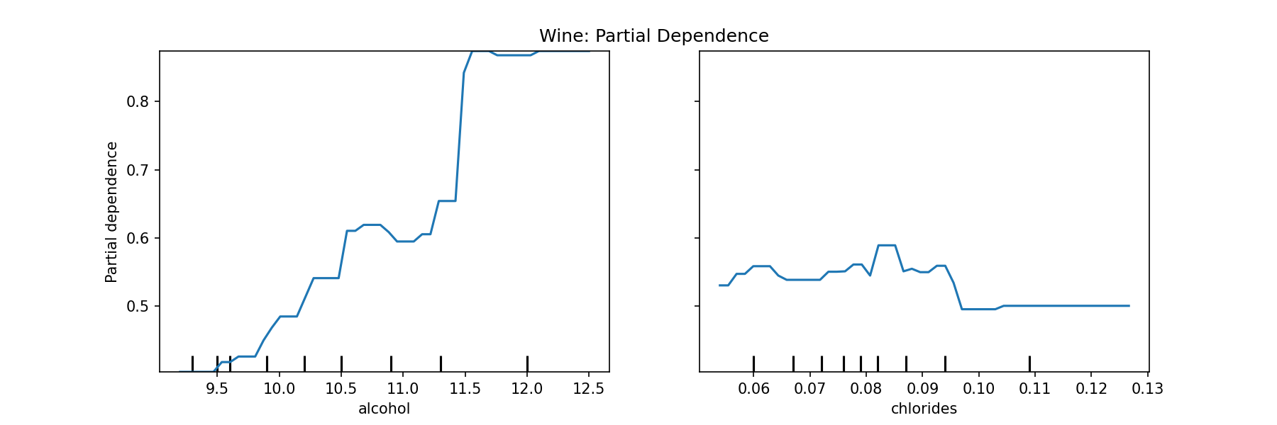
On the left plot, we can see that as the percentage of alcohol increases the model more strongly predicts higher quality. On the right, the amount of chlorides in the wine doesn't seem to affect the prediction as much as the alcohol content feature.
Now, we're going to use a different library to visualize the partial dependence for one feature. This plot is calculating the same dependence of the feature but is plotting all of the predictions (shaded area) as well as the average (solid line).
!pip install PDPbox

from pdpbox.pdp import PDPIsolate, PDPInteract
from pdpbox.info_plots import TargetPlot, InteractTargetPlot

isolated = PDPIsolate(
    model= wine_model,
    df=X,
    model_features=X.columns,
    feature='alcohol',
    feature_name='alcohol'
)
fig, axes = isolated.plot()
fig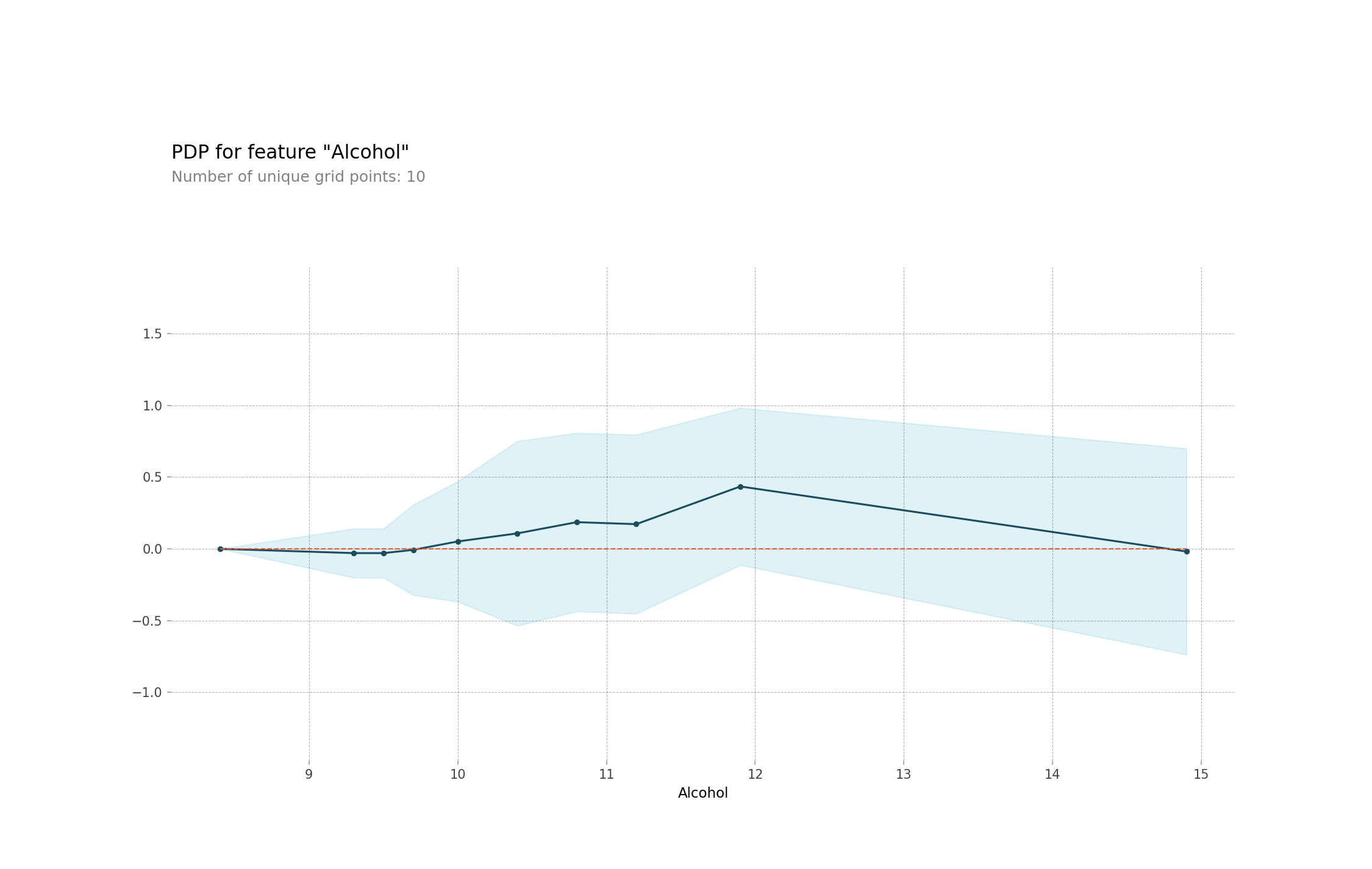
This plot is on a different scale that the first one but we can still see the same increase after 11% alcohol content.
Challenge
From the above example, select a different feature (or features) and re-create the plots above. Write out a few sentences to describe the dependence of the model prediction on that feature. Is the model affected by changes in the feature's values?
Additional Resources
Objective 02 - Explain individual predictions with shapley value plots
Overview
In this objective, we'll dive a little deeper into how individual features contribute to making a prediction. A quantity called a Shapley value, borrowed from the concept of game theory, will be used to explain the difference between the prediction of an individual observation and the average prediction from all the observations (instances).
One way to consider this problem is to think of all features in the model, that are working together to make a prediction. For example, using the wine data set from the previous objective, we can consider the alcohol content, the sulphates, and the pH. For one observation (row of the DataFrame) they work together to make a prediction. The rest of the rows all work together to make the average prediction. The Shapley values look at each feature's contribution to the single row prediction and explain exactly how it is different from the average prediction.
Let's work through an example using the SHAP library which stands for SHapley Additive exPlanations.
Follow Along
# Load the dataset
import pandas as pd
wine = pd.read_csv('winequality-red.csv')
wine.head()

# Set the features list and target variable
target = 'quality'
X = wine.drop(target, axis=1)

# Create the target array
y = wine['quality']

# Map the target to a binary class at quality = 5
y = y.apply(lambda x: 0 if x <= 5 else 1)
To calculate the Shapley values, we'll be fitting a xgboost classifier model to the data. The
TreeExplainer() is used to explain the output of ensemble tree models. From the explainer
values, we calculate the Shapley values and then visualize the results for a single observation
(instance).
# import shap
import shap

# Instantiate and fit the model
from xgboost import XGBClassifier
xgb = XGBClassifier(random_state=42)
wine_model = xgb.fit(X, y)

# Shap explainer initilization
shap_ex = shap.TreeExplainer(wine_model)

# Determine Shap values
shap_values = shap_ex.shap_values(X)
import matplotlib.pyplot as plt
# Calculate the shapley values
shap_values = shap_ex.shap_values(X)
# Initialize the plot
shap.initjs()
shap.force_plot(shap_ex.expected_value, shap_values[25,:], X.iloc[25,:])
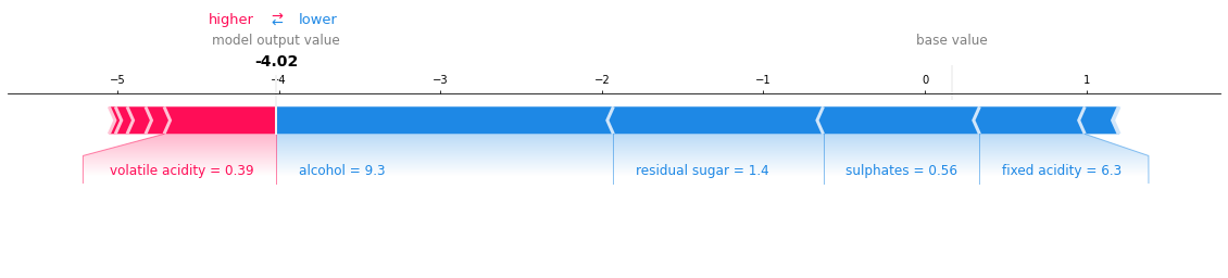
We can interpret the above plot in the following way: For the sample in 25th row, higher volatile acidity helped improve the wine quality, whereas a higher alcohol content and residual sugar (and others) resulted in lowering the quality of wine.
Challenge
We plotted the feature contributions for a single observation. Using the same code as above, try
selecting a different observation or row of the data frame. You might consider changing the value of
25 in shap_values[25,:] and X.iloc[25,:]. Write out a few
sentences to describe what the SHAP plot
indicates about the feature contributions for this observation.
Additional Resources
Guided Project
Open DS_234_guided_project_notes.ipynb in the GitHub repository below to follow along with the guided project:
Guided Project Video - Part One
Guided Project Video - Part Two
Module Assignment
For this final assignment, you'll apply model interpretation techniques to your portfolio project to gain insights and effectively communicate your model's behavior.
Note: There is no video for this assignment as you will be working with your own dataset and defining your own machine learning problem.