Module 1: Define ML Problems
Module Overview
In this module, you'll learn how to properly define machine learning problems. This is a crucial first step in any data science project, as a well-defined problem sets the foundation for all subsequent modeling decisions. You'll learn to choose appropriate targets, understand their distributions, and select evaluation metrics that align with your project goals.
Learning Objectives
- choose a target to predict, and check its distribution
- avoid leakage of information from test to train or from target to features
- choose an appropriate evaluation metric
- use the classification metric ROC AUC to interpret a classifier model
Objective 01 - Choose a target to predict, and check its distribution
Overview
Up to this point in the course we have worked with a lot of data sets and fit a number of different types of models to those data sets. While this has been helpful practice for learning how to select a model, create pipelines, and evaluate the results, we could use some additional experience with data that is generally less "prepared."
Working through the example in this objective will give us a chance to more carefully consider our target. We should be looking at the distribution of the target and its suitability for modeling; if the classes are balanced, the appropriate type of encoding to use, and how that choice might affect the model.
In the next section, we'll be using a data set from Kaggle. While this data is mostly prepared for machine learning, it's still important to think about the target and what we are trying to model.
Follow Along
This data set is available on here. It records observations of Australian weather in order to try to predict if rain occurred on the day following the measurements.
# Import libraries, load data, and view
import pandas as pd
url="https://raw.githubusercontent.com/bloominstituteoftechnology/DS-Unit-2-Kaggle-Challenge/main/data/weather/weatherAUS.csv"
weather=pd.read_csv(url)
weather.head()| Date | Location | MinTemp | MaxTemp | Rainfall | Evaporation | Sunshine | WindGustDir | WindGustSpeed | WindDir9am | ... | Humidity3pm | Pressure9am | Pressure3pm | Cloud9am | Cloud3pm | Temp9am | Temp3pm | RainToday | RISK_MM | RainTomorrow | |
|---|---|---|---|---|---|---|---|---|---|---|---|---|---|---|---|---|---|---|---|---|---|
| 0 | 2008-12-01 | Albury | 13.4 | 22.9 | 0.6 | NaN | NaN | W | 44.0 | W | ... | 22.0 | 1007.7 | 1007.1 | 8.0 | NaN | 16.9 | 21.8 | No | 0.0 | No |
| 1 | 2008-12-02 | Albury | 7.4 | 25.1 | 0.0 | NaN | NaN | WNW | 44.0 | NNW | ... | 25.0 | 1010.6 | 1007.8 | NaN | NaN | 17.2 | 24.3 | No | 0.0 | No |
| 2 | 2008-12-03 | Albury | 12.9 | 25.7 | 0.0 | NaN | NaN | WSW | 46.0 | W | ... | 30.0 | 1007.6 | 1008.7 | NaN | 2.0 | 21.0 | 23.2 | No | 0.0 | No |
| 3 | 2008-12-04 | Albury | 9.2 | 28.0 | 0.0 | NaN | NaN | NE | 24.0 | SE | ... | 16.0 | 1017.6 | 1012.8 | NaN | NaN | 18.1 | 26.5 | No | 1.0 | No |
| 4 | 2008-12-05 | Albury | 17.5 | 32.3 | 1.0 | NaN | NaN | W | 41.0 | ENE | ... | 33.0 | 1010.8 | 1006.0 | 7.0 | 8.0 | 17.8 | 29.7 | No | 0.2 | No |
5 rows × 24 columns
As we typically do with a data set, we should get some more details. We can use the
df.info() method
to
see how many columns we have, the data types for each of those columns, and how many of those values
are
non-null.
# Display the info for the weather DataFrame
weather.info()
<class 'pandas.core.frame.DataFrame'>
RangeIndex: 142193 entries, 0 to 142192
Data columns (total 24 columns):
# Column Non-Null Count Dtype
--- ------ -------------- -----
0 Date 142193 non-null object
1 Location 142193 non-null object
2 MinTemp 141556 non-null float64
3 MaxTemp 141871 non-null float64
4 Rainfall 140787 non-null float64
5 Evaporation 81350 non-null float64
6 Sunshine 74377 non-null float64
7 WindGustDir 132863 non-null object
8 WindGustSpeed 132923 non-null float64
9 WindDir9am 132180 non-null object
10 WindDir3pm 138415 non-null object
11 WindSpeed9am 140845 non-null float64
12 WindSpeed3pm 139563 non-null float64
13 Humidity9am 140419 non-null float64
14 Humidity3pm 138583 non-null float64
15 Pressure9am 128179 non-null float64
16 Pressure3pm 128212 non-null float64
17 Cloud9am 88536 non-null float64
18 Cloud3pm 85099 non-null float64
19 Temp9am 141289 non-null float64
20 Temp3pm 139467 non-null float64
21 RainToday 140787 non-null object
22 RISK_MM 142193 non-null float64
23 RainTomorrow 142193 non-null object
dtypes: float64(17), object(7)
memory usage: 26.0+ MBThere are definitely missing values in some of the columns. There are also columns labeled
date but
since
they are object type, they will need to be converted to datetime objects.
Additionally, we have
quite a
few categorical variables that will need to be either labeled or encoded. Finally and most
importantly,
we need to figure out what we are trying to predict from this data set!
The variables in this data set relate to measurements of the weather such as temperature, wind speed
and
direction, atmospheric pressure, and if there was rain on that current date. The feature that
suggests
something like a prediction is RainTomorrow. This column contains an object
data type and
when we
look
at the column values in more detail, we can see the values are categorical ('Yes' and 'No').
Let's take a look at our potential target and how the 'Yes' and 'No' classes are distributed.
# Look at the 'outcome_type' column
weather['RainTomorrow'].value_counts()
No 110316
Yes 31877
Name: RainTomorrow, dtype: int64# Look at the 'outcome_type' column
weather['RainTomorrow'].value_counts(normalize=True)No 0.775819
Yes 0.224181
Name: RainTomorrow, dtype: float64This target has two somewhat imbalanced classes with 78% 'Yes' and 22% 'No' but will work fine as an example classification task. When we have imbalanced data, there are different ways to address possible problems, including using different metrics to evaluate the model. The topic of imbalanced data will likely come up (if it hasn't already!) as you work through both the Guided Projects and the Module Projects.
Challenge
For the Module Project, you will source your own data set and fit a model. As you are searching for something to work with, take a few minutes to look at each data set you come across and think about what the target variable would be. One stipulation for this exercise: try to find a data set where the target is not already specified. You don't need to perform any analysis right now other than viewing the data and making some effort to understand the features.
Additional Resources
Data Science Is Not Taught At Universities - And Here Is Why
Objective 02 - Avoid leakage of information from test to train or from target to features
Overview
We briefly introduced the concept of data leakage in the previous sprint when we discussed using pipelines for preprocessing and model fitting. In general, and especially if you are using cross-validation, it's good to be conscious of when, where, and why data leakage can occur. This module is focused on learning how to work with data that isn't already prepared for modeling. Not only do we need to know which features to use and if our target is appropriate, but we also need to protect against information leaking into either our testing data or from certain features.
The two main types of leakage are leaky features (predictors) and a leaky validation or testing process.
Leaky Features
This type of leakage occurs when you have a feature that has access to data that won't be available when you actually use the model on new data (outside of the test set) to make predictions. This could happen if you adjust the values in that feature after you determined the values in your target array.
For example, if we were predicting if someone has heart disease (True/False) and used a feature called
BP_meds (indicating if the individual is taking blood pressure medication), we might have a
problem. If
someone is taking this medication, it might be because they have heart disease and are being treated.
Moreover, the value in this column could have been changed after they were diagnosed with heart disease.
Leaky Testing Process
The other type of leak can happen when your validation data "learns" from the training data. If you are
preprocessing the data, such as filling in missing values with the SimpleImputer or
standardizing values with StandardScaler, you might accidentally be using the entire data
set. In this case, it's important
to apply the preprocessing steps separately to the training and testing data which will prevent the
testing data from learning anything from the training set.
Now that we are more familiar with these two different types of data leakage, let's explore our real-world weather data from the previous objective.
Follow Along
We introduced the Australian weather data set earlier and explored it briefly to decide on the prediction target: whether it was going to rain on the day following the measurements. Let's look more closely at each of the features (predictors) to see if any of them could present leakage problems.
#Import libraries, load data, and view
import pandas as pd
url="https://raw.githubusercontent.com/bloominstituteoftechnology/DS-Unit-2-Kaggle-Challenge/main/data/weather/weatherAUS.csv"
weather=pd.read_csv(url)
weather.head()| Date | Location | MinTemp | MaxTemp | Rainfall | Evaporation | Sunshine | WindGustDir | WindGustSpeed | WindDir9am | ... | Humidity3pm | Pressure9am | Pressure3pm | Cloud9am | Cloud3pm | Temp9am | Temp3pm | RainToday | RISK_MM | RainTomorrow | |
|---|---|---|---|---|---|---|---|---|---|---|---|---|---|---|---|---|---|---|---|---|---|
| 0 | 2008-12-01 | Albury | 13.4 | 22.9 | 0.6 | NaN | NaN | W | 44.0 | W | ... | 22.0 | 1007.7 | 1007.1 | 8.0 | NaN | 16.9 | 21.8 | No | 0.0 | No |
| 1 | 2008-12-02 | Albury | 7.4 | 25.1 | 0.0 | NaN | NaN | WNW | 44.0 | NNW | ... | 25.0 | 1010.6 | 1007.8 | NaN | NaN | 17.2 | 24.3 | No | 0.0 | No |
| 2 | 2008-12-03 | Albury | 12.9 | 25.7 | 0.0 | NaN | NaN | WSW | 46.0 | W | ... | 30.0 | 1007.6 | 1008.7 | NaN | 2.0 | 21.0 | 23.2 | No | 0.0 | No |
| 3 | 2008-12-04 | Albury | 9.2 | 28.0 | 0.0 | NaN | NaN | NE | 24.0 | SE | ... | 16.0 | 1017.6 | 1012.8 | NaN | NaN | 18.1 | 26.5 | No | 1.0 | No |
| 4 | 2008-12-05 | Albury | 17.5 | 32.3 | 1.0 | NaN | NaN | W | 41.0 | ENE | ... | 33.0 | 1010.8 | 1006.0 | 7.0 | 8.0 | 17.8 | 29.7 | No | 0.2 | No |
5 rows × 24 columns
Before we identify any possible "leaky features" we should decide which features to use and the necessary preprocessing steps. Let's look at each type of variable (numeric and categorical) in more detail.
# Look at the statistics of categorical variables
weather.describe(include=['object'])| Date | Location | WindGustDir | WindDir9am | WindDir3pm | RainToday | RainTomorrow | |
|---|---|---|---|---|---|---|---|
| count | 142193 | 142193 | 132863 | 132180 | 138415 | 140787 | 142193 |
| unique | 3436 | 49 | 16 | 16 | 16 | 2 | 2 |
| top | 2013-10-08 | Canberra | W | N | SE | No | No |
| freq | 49 | 3418 | 9780 | 11393 | 10663 | 109332 | 110316 |
# Look at the statistics of the numeric variables
weather.describe()| MinTemp | MaxTemp | Rainfall | Evaporation | Sunshine | WindGustSpeed | WindSpeed9am | WindSpeed3pm | Humidity9am | Humidity3pm | Pressure9am | Pressure3pm | Cloud9am | Cloud3pm | Temp9am | Temp3pm | RISK_MM | |
|---|---|---|---|---|---|---|---|---|---|---|---|---|---|---|---|---|---|
| count | 141556.000000 | 141871.000000 | 140787.000000 | 81350.000000 | 74377.000000 | 132923.000000 | 140845.000000 | 139563.000000 | 140419.000000 | 138583.000000 | 128179.000000 | 128212.000000 | 88536.000000 | 85099.000000 | 141289.000000 | 139467.000000 | 142193.000000 |
| mean | 12.186400 | 23.226784 | 2.349974 | 5.469824 | 7.624853 | 39.984292 | 14.001988 | 18.637576 | 68.843810 | 51.482606 | 1017.653758 | 1015.258204 | 4.437189 | 4.503167 | 16.987509 | 21.687235 | 2.360682 |
| std | 6.403283 | 7.117618 | 8.465173 | 4.188537 | 3.781525 | 13.588801 | 8.893337 | 8.803345 | 19.051293 | 20.797772 | 7.105476 | 7.036677 | 2.887016 | 2.720633 | 6.492838 | 6.937594 | 8.477969 |
| min | -8.500000 | -4.800000 | 0.000000 | 0.000000 | 0.000000 | 6.000000 | 0.000000 | 0.000000 | 0.000000 | 0.000000 | 980.500000 | 977.100000 | 0.000000 | 0.000000 | -7.200000 | -5.400000 | 0.000000 |
| 25% | 7.600000 | 17.900000 | 0.000000 | 2.600000 | 4.900000 | 31.000000 | 7.000000 | 13.000000 | 57.000000 | 37.000000 | 1012.900000 | 1010.400000 | 1.000000 | 2.000000 | 12.300000 | 16.600000 | 0.000000 |
| 50% | 12.000000 | 22.600000 | 0.000000 | 4.800000 | 8.500000 | 39.000000 | 13.000000 | 19.000000 | 70.000000 | 52.000000 | 1017.600000 | 1015.200000 | 5.000000 | 5.000000 | 16.700000 | 21.100000 | 0.000000 |
| 75% | 16.800000 | 28.200000 | 0.800000 | 7.400000 | 10.600000 | 48.000000 | 19.000000 | 24.000000 | 83.000000 | 66.000000 | 1022.400000 | 1020.000000 | 7.000000 | 7.000000 | 21.600000 | 26.400000 | 0.800000 |
| max | 33.900000 | 48.100000 | 371.000000 | 145.000000 | 14.500000 | 135.000000 | 130.000000 | 87.000000 | 100.000000 | 100.000000 | 1041.000000 | 1039.600000 | 9.000000 | 9.000000 | 40.200000 | 46.700000 | 371.000000 |
Data Exploration: Null Values
From the above DataFrame descriptions we can see that there are a lot of null values in some of the columns. We'll take a more detailed look at how many are missing in what columns. The plot below is created using a module available at this repository.
# Checking for null values
weather.isnull().sum()
Date 0
Location 0
MinTemp 637
MaxTemp 322
Rainfall 1406
Evaporation 60843
Sunshine 67816
WindGustDir 9330
WindGustSpeed 9270
WindDir9am 10013
WindDir3pm 3778
WindSpeed9am 1348
WindSpeed3pm 2630
Humidity9am 1774
Humidity3pm 3610
Pressure9am 14014
Pressure3pm 13981
Cloud9am 53657
Cloud3pm 57094
Temp9am 904
Temp3pm 2726
RainToday 1406
RISK_MM 0
RainTomorrow 0import matplotlib.pyplot as plt
import missingno as msno
msno.matrix(weather)
plt.show()
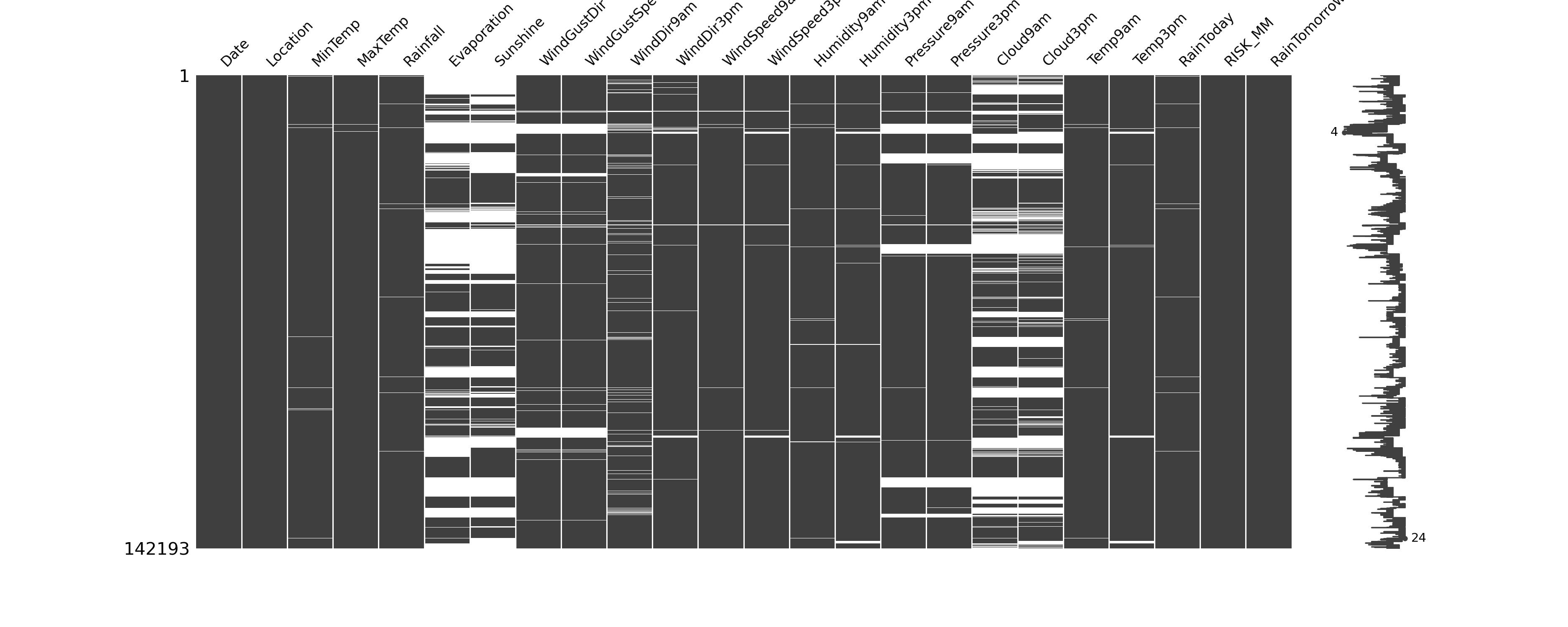
We have four columns with a large number of null values. If we were doing this analysis for a competition
(or for an actual data science job!) we would want to more carefully explore the missing values. Since
these columns are missing about 40% of their data (or more), we're going to drop them for this analysis.
For the other missing values, we'll use an Imputer in the preprocessing step.
To simplify the analysis for later, we'll also drop the Location column. Again, this
information might be
important for a more detailed model, but we're trying to keep this process simple so that we can focus
on identifying the leaky features.
# Drop columns with high-percentage of missing values
cols_drop = ['Location', 'Evaporation', 'Sunshine', 'Cloud9am', 'Cloud3pm']
weather_drop = weather.drop(cols_drop, axis=1)
Data Cleaning: Datetime
We have a date column which could be converted to a datetime object. We will use only the 'month' value from this column in our model, as the full date would be too specific.
# Convert the 'Date' column to datetime, extract month
weather_drop['Date'] = pd.to_datetime(weather_drop['Date'], infer_datetime_format=True).dt.month
weather_drop.head()
Data Processing: Pipeline
We'll separate our features into numeric and categorical types and then perform transformation steps.
Several of the numeric features are on very different scales, so we will standardize those values. We
will also impute our missing values with SimpleImputer(). The categorical features will be
ordinarily encoded.
# Print the column names
weather_drop.columns
# Imports
import pandas as pd
import numpy as np

from sklearn.compose import ColumnTransformer
from sklearn.pipeline import Pipeline
from sklearn.impute import SimpleImputer
from sklearn.preprocessing import StandardScaler, OrdinalEncoder
from sklearn.linear_model import LogisticRegression
from sklearn.tree import DecisionTreeClassifier

# Define the numeric features
numeric_features = ['MinTemp', 'MaxTemp', 'Rainfall', 'WindGustSpeed',
                    'WindSpeed9am','WindSpeed3pm', 'Humidity9am',
                    'Humidity3pm', 'Pressure9am','Pressure3pm',
                    'Temp9am', 'Temp3pm', 'RISK_MM']

# Create the transformer (impute, scale)
numeric_transformer = Pipeline(steps=[
    ('imputer', SimpleImputer(strategy='median')),
    ('scaler', StandardScaler())])

# Define the categorical features
categorical_features = ['WindGustDir', 'WindDir9am', 'WindDir3pm', 'RainToday']
categorical_transformer = Pipeline(steps=[
    ('imputer', SimpleImputer(strategy='constant', fill_value='missing')),
    ('ordinal', OrdinalEncoder())])

# Define how the numeric and categorical features will be transformed
preprocessor = ColumnTransformer(
    transformers=[
        ('num', numeric_transformer, numeric_features),
        ('cat', categorical_transformer, categorical_features)])

# Define the pipeline steps, including the classifier
clf = Pipeline(steps=[('preprocessor', preprocessor),
                  ('classifier', DecisionTreeClassifier())])
Create Feature Matrix, Target Array
We have a couple of final steps before we fit the model: create the feature matrix and then create and encode the target array.
# Create the feature matrix
X = weather_drop.drop('RainTomorrow', axis=1)

# Create and encode the target array
from sklearn.preprocessing import LabelEncoder
label_enc = LabelEncoder()
y=label_enc.fit_transform(weather_drop['RainTomorrow'])
# Import the train_test_split utility
from sklearn.model_selection import train_test_split

# Create the training and test sets
X_train, X_test, y_train, y_test = train_test_split(
    X, y, test_size=0.2, random_state=42)
# Fit the model
clf.fit(X_train,y_train)
print('Validation Accuracy', clf.score(X_test, y_test))
Wow! We achieved 100% accuracy. Is this too good to be true? Yes - anytime you have a model with very high accuracy you likely have a problem and that problem is probably data leakage of some type. Let's look at the feature importances to see where the problem is.
# Features (order in which they were preprocessed)
features_order = numeric_features + categorical_features

# Determine the importances
importances = pd.Series(clf.steps[1][1].feature_importances_, features_order)
# Plot feature importances
import matplotlib.pyplot as plt

n = 7
plt.figure(figsize=(10,n/2))
plt.title(f'Top {n} features')
importances.sort_values()[-n:].plot.barh(color='grey')

plt.show()
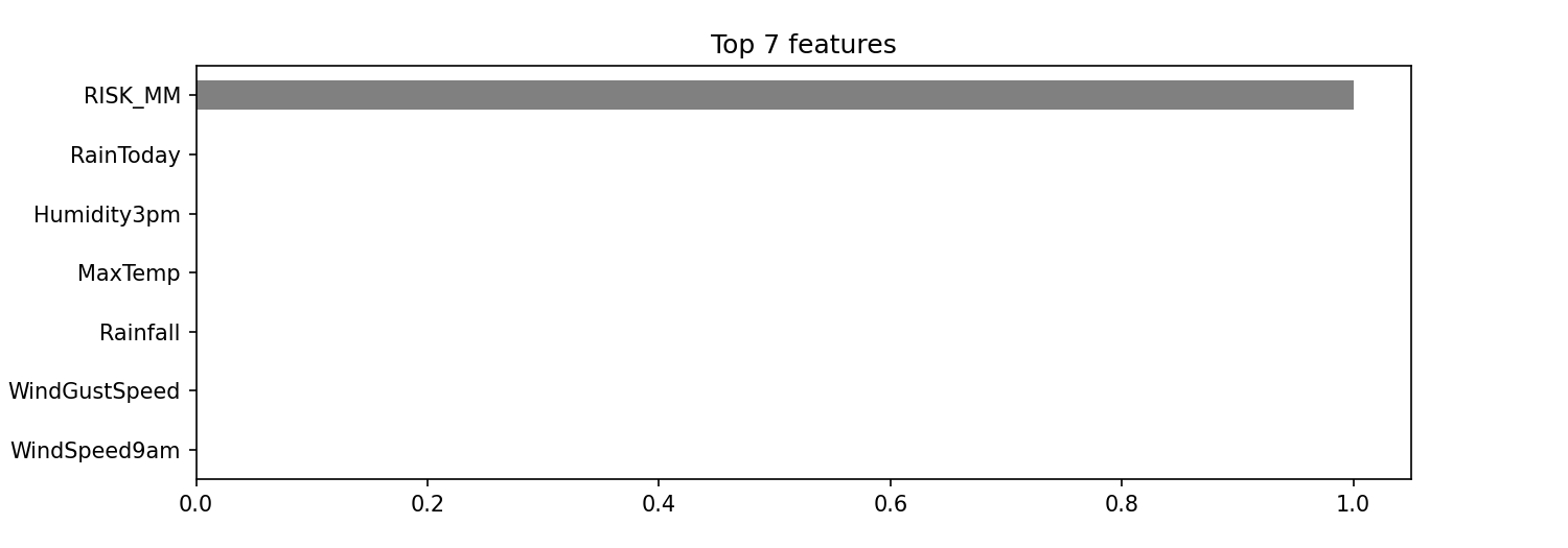
It looks like the model was essentially fit on a single feature, which must be because the predictor was
related to the target array. Spoiler: one of the features is leaking information to the model. It is the
RISK_MM column which is essentially how much rain was recorded the following day.
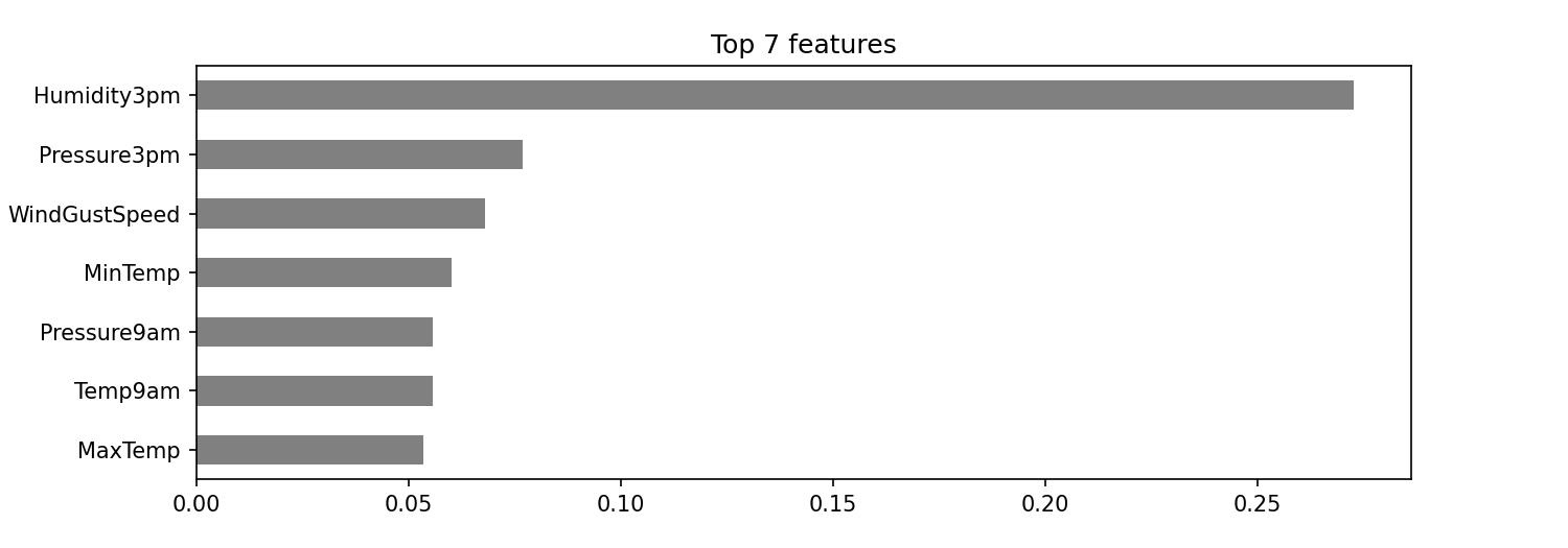
We'll remove this column, run the model again, and calculate the features importances.
# Remove the 'RISK_MM' column
X_noriskmm = X.drop('RISK_MM', axis=1)

# Create the new training and test sets
X_train, X_test, y_train, y_test = train_test_split(
    X_noriskmm, y, test_size=0.2, random_state=42)

# Drop the 'RISK_MM' column from the numeric_features
numeric_features = numeric_features.remove('RISK_MM')

# Fit the model
clf.fit(X_train,y_train)
print('Validation Accuracy (with no "RISK_MM")', clf.score(X_test, y_test))
That's better! The accuracy is still high, but much more reasonable.
# Get feature importances

# Features (order in which they were preprocessed)
numeric_features = ['MinTemp', 'MaxTemp', 'Rainfall', 'WindGustSpeed',
                    'WindSpeed9am','WindSpeed3pm', 'Humidity9am',
                    'Humidity3pm', 'Pressure9am','Pressure3pm',
                    'Temp9am', 'Temp3pm']

categorical_features = ['WindGustDir', 'WindDir9am', 'WindDir3pm', 'RainToday']
features_order = numeric_features + categorical_features

importances = pd.Series(clf.steps[1][1].feature_importances_, features_order)
# Plot feature importances
n = 7
plt.figure(figsize=(10,n/2))
plt.title(f'Top {n} features')
importances.sort_values()[-n:].plot.barh(color='grey')
plt.clf()
Challenge
In the above example, we removed the RISK_MM column. However, this takes away information
that we might
use in our model. For this challenge, think of a way you could group the values in this column and use
it as the target for the model. Can we predict how much rain is received instead of just a true/false
prediction?
Additional Resources
Objective 03 - Choose an appropriate evaluation metric
Overview
Up to this point in the course we've fit several different models: linear regression, logistic regression, decision tree, and random forests. One concept that we haven't covered extensively is how to choose the metric by which we evaluate our models.
Because it's important, the following information is likely to be repeated during the Guided Project:
Classification & regression metrics are different!
- Don't use regression metrics to evaluate classification tasks.
- Don't use classification metrics to evaluate regression tasks.
Let's look at each type of task and the associated metrics.
Classification Tasks
For classification tasks we can use the metrics of: precision, recall, F1 score, and the receiver operating characteristic (ROC) curve. Some general rules to follow when choosing one of these metrics:
- accuracy is useful when the majority class is between 50-70%
- precision and recall can be helpful for finding misclassified observations
- ROC curve is helpful for when you need probabilities associated with your predictions
Regression Tasks
Generally, regression models are scored by the R squared value. It is the proportion of the variance in the dependent variable (y) that is predictable from the independent variable(s) (X).
We'll use the iris data set here to do a basic evaluation metric exercise.
Follow Along
Let's load in the data, create the training and test sets, fit the model, and, finally, evaluate our model.
# Load in libraries, data
from sklearn import datasets, metrics
from sklearn.model_selection import train_test_split

# Create X, y and training/test sets
iris = datasets.load_iris()
X = iris.data
y = iris.target

X_train, X_test, y_train, y_test = train_test_split(
    X, y, test_size=0.4, random_state=42)

# Import the classifier
from sklearn.tree import DecisionTreeClassifier

dt_classifier = DecisionTreeClassifier(random_state=42)
dt_classifier.fit(X_train,y_train)

print('Validation Accuracy: ', dt_classifier.score(X_test, y_test))
Validation Accuracy: 0.9666666666666667This model has a pretty high accuracy, so let's look at a few other metrics which might give us a better idea of how the model is fitting the data. First, we'll create a visualization of the confusion matrix.
# import matplotlib.pyplot as plt
from sklearn.metrics import ConfusionMatrixDisplay

ConfusionMatrixDisplay.from_estimator(dt_classifier, X_test, y_test)
plt.show()
<Figure size 576x576 with 0 Axes>
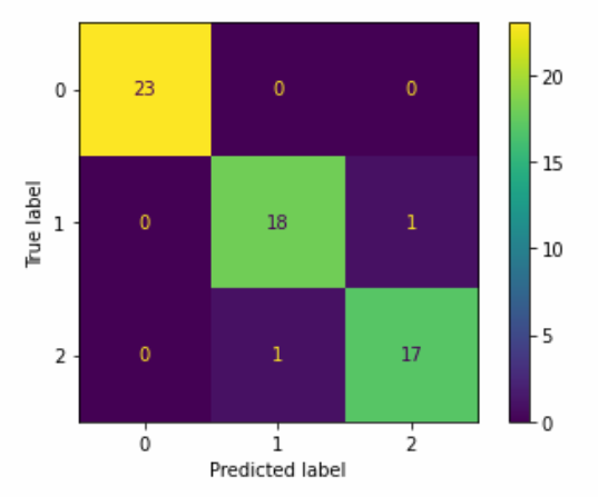
We can see from the confusion matrix that very few of the observations are being misclassified, so the high accuracy is probably correct for this model.
We can also look at the classification report, which shows the precision, recall, and the F1-score.
# Create the classification report
y_pred = dt_classifier.predict(X_test)
print(metrics.classification_report(y_test, y_pred))
              precision    recall  f1-score   support

           0       1.00      1.00      1.00        23
           1       0.95      0.95      0.95        19
           2       0.94      0.94      0.94        18

    accuracy                           0.97        60
   macro avg       0.96      0.96      0.96        60
weighted avg       0.97      0.97      0.97        60
Challenge
For this challenge, think about a data set you have worked with that you haven't yet evaluated. Which metric should you use? Do you understand how the model is being evaluated?
Additional Resources
Objective 04 - Use the classification metric ROC AUC to interpret a classifier model
Overview
In the previous sprint, we examined the probability threshold a classifier uses when determining the class to which an observation belongs. We can extend this concept and look at something called the receiver operating characteristic, which is usually plotted as a curve and called the ROC curve.
First, we'll go back to the idea of calculating true positives and true negatives and look at a different measurement, the true positive rate (TPR) and the false positive rate (FPR).
Both of the above measurements are the total true or false positives normalized by the total for each.
When we create a ROC curve, we are plotting the TPR against the FPR for a range of threshold values. In
the next section, we'll use the scikit-learn roc_curve() method to do the calculations for
us. From the
resulting data, we'll create a plot.
Follow Along
In order to plot a ROC curve, we need some data and a classifier model fit to that data. Let's create some data from the previous objective and then build the ROC curve.
# Load modules
import pandas as pd
from sklearn.datasets import make_classification
from sklearn.linear_model import LogisticRegression
from sklearn.model_selection import train_test_split
from sklearn.metrics import roc_curve

# Create the data (feature, target)
X, y = make_classification(n_samples=10000, n_features=5,
                          n_classes=2, n_informative=3,
                          random_state=42)

# Split the data into a training set and a test set
X_train, X_test, y_train, y_test = train_test_split(X, y, random_state=42)

# Create and fit the model
logreg_classifier = LogisticRegression().fit(X_train, y_train)

# Create predicted probabilities
y_pred_prob = logreg_classifier.predict_proba(X_test)[:,1]
# Create the data for the ROC curve
fpr, tpr, thresholds = roc_curve(y_test, y_pred_prob)

# See the results in a table
roccurve_df = pd.DataFrame({
    'False Positive Rate': fpr,
    'True Positive Rate': tpr,
    'Threshold': thresholds
})

roccurve_df.head()| False Positive Rate | True Positive Rate | Threshold | |
|---|---|---|---|
| 0 | 0.000000 | 0.000000 | 1.999969 |
| 1 | 0.000000 | 0.000786 | 0.999969 |
| 2 | 0.000000 | 0.291438 | 0.983222 |
| 3 | 0.000815 | 0.291438 | 0.983049 |
| 4 | 0.000815 | 0.360566 | 0.970583 |
# Plot the ROC curve
import matplotlib.pyplot as plt

plt.plot(fpr, tpr)
plt.plot([0,1], ls='--')
plt.title('ROC curve')
plt.xlabel('False Positive Rate')
plt.ylabel('True Positive Rate')

plt.show()
<Figure size 432x288 with 0 Axes>
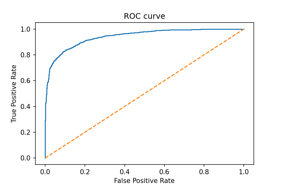
The above model looks pretty good. In general, the better a model, the higher the curve is, and the greater the area under the curve (AUC). The maximum value for the AUC is equal to one. While we can "eyeball" the area in our curve, there is also a tool used to calculate the AUC.
# Calculate the area under the curve
from sklearn.metrics import roc_auc_score
roc_auc_score(y_test, y_pred_prob)
0.9419681927513379
Challenge
Using a different data set for classification, see if you can construct the ROC curve. Or with the same data set generated above, try using a different classifier such as a decision tree and plot the ROC curve and calculate the AUC. Which model performs better?
Additional Resources
Guided Project
Open DS_231_guided_project.ipynb in the GitHub repository below to follow along with the guided project:
Guided Project Video
Module Assignment
For this assignment, you'll apply what you've learned to your own portfolio dataset. This hands-on experience will solidify your understanding of the concepts and prepare you for real-world machine learning tasks.
Note: There is no video solution for this assignment as you will be working with your own dataset and defining your own machine learning problem.