Module 3: Permutation and Boosting
Module Overview
In this module, you'll learn about ensemble methods with a focus on bagging and boosting techniques. You'll understand how gradient boosting models work and how to interpret feature importances through both default and permutation methods. These techniques will help you build more powerful models and gain deeper insights into what drives your predictions.
Learning Objectives
- Bagging vs. Boosting
- Gradient Boosting Model
- Feature Importances (default and permutation)
Objective 01 - Get permutation importances for model interpretation and feature selection
Overview
In many of the models we've fit, we've looked at the feature importance. This has been accomplished by ranking the features after fitting the model. In addition to these basic methods, we can also look at what happens when we change a specific feature. This is called permutation importance.
To permute something means to change the order. When we fit a model we measure the accuracy by comparing our model predictions to the test or validation data. We can test the importance of a feature by permuting the values and calculating the accuracy against the test set.
The process works something like this:
- Fit a model and calculate the accuracy on test set
- Choose a feature (by ranking the importances or some other method) and randomly permute the test set values for just that feature
- Calculate the accuracy on test set again with the permuted column
- If it results in a decrease in accuracy: that feature is important to the model
- If it results in an accuracy that stays the same: the feature isn't important to the model and could be replaced by random numbers
Follow Along
We'll use the Australian weather data set from the previous module and permute or randomize a few of the features in the test set. The accuracy should change, or decrease for features that are important to the model. Additionally, the accuracy should remain essentially the same for features that are not very important to the model.
# Import libraries, load data, and view
import pandas as pd
url = "https://raw.githubusercontent.com/bloominstituteoftechnology/DS-Unit-2-Kaggle-Challenge/main/data/weather/weatherAUS.csv"
weather = pd.read_csv(url)
weather.head()

# Drop columns with high-percentage of missing values (and the leaky feature)
cols_drop = ['Location', 'Evaporation', 'Sunshine', 'Cloud9am', 'Cloud3pm', 'RISK_MM']
weather_drop = weather.drop(cols_drop, axis=1)

# Convert the 'Date' column to datetime, extract month
weather_drop['Date'] = pd.to_datetime(weather_drop['Date'], infer_datetime_format=True).dt.month
Create Pipeline
Here we're going to create the preprocessing and model fitting pipeline from the first module in this sprint, so you have seen this code before! Once the model is fit, we can demonstrate the feature-permutation process.
# Imports
import pandas as pd
import numpy as np

from sklearn.compose import ColumnTransformer
from sklearn.pipeline import Pipeline
from sklearn.impute import SimpleImputer
from sklearn.preprocessing import StandardScaler, OrdinalEncoder
from sklearn.tree import DecisionTreeClassifier


# Define the numeric features
numeric_features = ['MinTemp', 'MaxTemp', 'Rainfall', 'WindGustSpeed',
                    'WindSpeed9am','WindSpeed3pm', 'Humidity9am',
                    'Humidity3pm', 'Pressure9am','Pressure3pm',
                    'Temp9am', 'Temp3pm']

# Create the transformer (impute, scale)
numeric_transformer = Pipeline(steps=[
    ('imputer', SimpleImputer(strategy='median')),
    ('scaler', StandardScaler())])

# Define the categorical features
categorical_features = ['WindGustDir', 'WindDir9am', 'WindDir3pm', 'RainToday']
categorical_transformer = Pipeline(steps=[
    ('imputer', SimpleImputer(strategy='constant', fill_value='missing')),
    ('ordinal', OrdinalEncoder())])

# Define how the numeric and categorical features will be transformed
preprocessor = ColumnTransformer(
    transformers=[
        ('num', numeric_transformer, numeric_features),
        ('cat', categorical_transformer, categorical_features)])

# Define the pipeline steps, including the classifier
clf = Pipeline(steps=[('preprocessor', preprocessor),
                  ('classifier', DecisionTreeClassifier())])
Train and Fit the Model
# Create the feature matrix
X = weather_drop.drop('RainTomorrow', axis=1)

# Create and encode the target array
from sklearn.preprocessing import LabelEncoder
label_enc = LabelEncoder()
y=label_enc.fit_transform(weather_drop['RainTomorrow'])

# Import the train_test_split utility
from sklearn.model_selection import train_test_split

# Create the training and test sets
X_train, X_test, y_train, y_test = train_test_split(
    X, y, test_size=0.2, random_state=42)

# Fit the model
clf.fit(X_train,y_train)
print('Validation Accuracy', clf.score(X_test, y_test))
Validation Accuracy 0.7793522979007701Feature Importances
We're looking at the feature importances now (after removing the problematic leaky feature). This is important because we need to see how the features rank before we change them around.
# Features (order in which they were preprocessed)
features_order = numeric_features + categorical_features

importances = pd.Series(clf.steps[1][1].feature_importances_, features_order)

# Plot feature importances
import matplotlib.pyplot as plt

n = 10
plt.figure(figsize=(10,n/2))
plt.title(f'Top {n} features')
importances.sort_values()[-n:].plot.barh(color='grey')

plt.show()
<Figure size 720x360 with 0 Axes>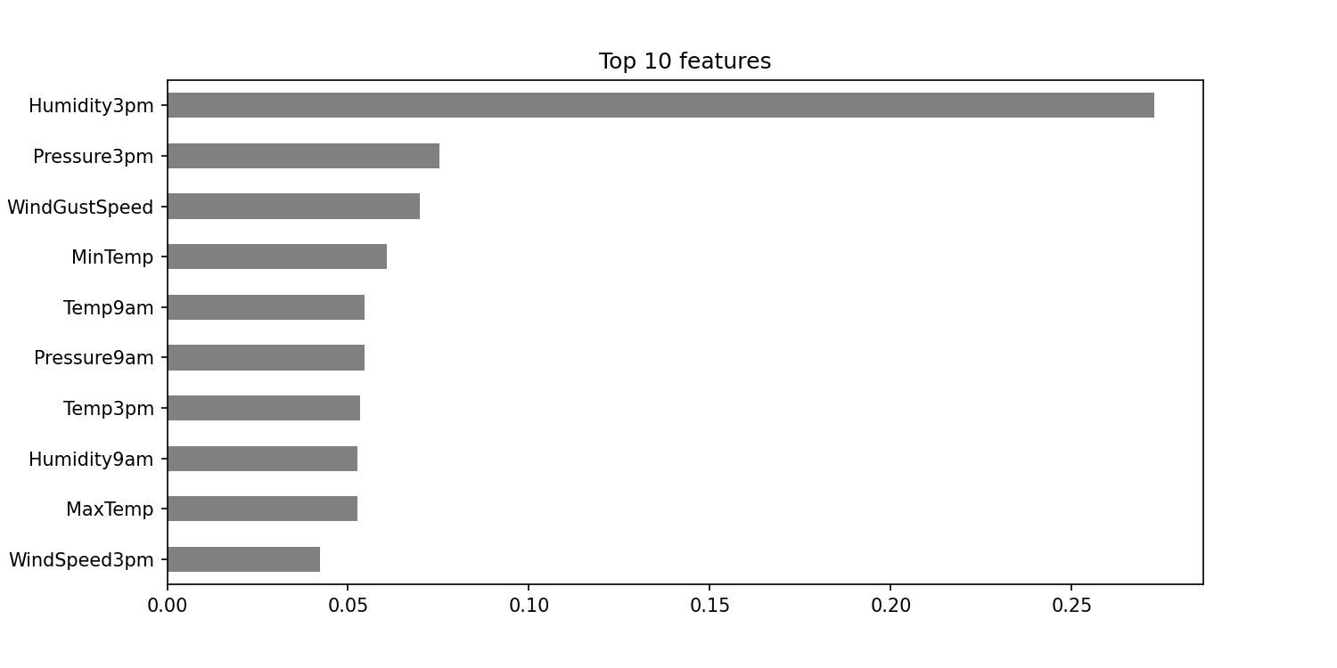
We can now try a few of the columns and see how permutation of their values affects the accuracy. We'll
start with the most important feature (Humidity3pm) and then do the same with one of the
less important features (WindSpeed3pm).
We need to remember to preprocess the permuted data in the same way we did inside of the pipeline above.
For the numeric features, we used SimpleImputer() and StandardScaler().
# Permute the values in the more important column
feature = 'Humidity3pm'
X_test_permuted = X_test.copy()

# Fill in missing values
X_test_permuted[feature].fillna(value = X_test_permuted[feature].median(), inplace=True)

# Permute
X_test_permuted[feature] = np.random.permutation(X_test[feature])

print('Feature permuted: ', feature)
print('Validation Accuracy', clf.score(X_test, y_test))
print('Validation Accuracy (permuted)', clf.score(X_test_permuted, y_test))
Feature permuted: Humidity3pm
Validation Accuracy 0.7793522979007701
Validation Accuracy (permuted) 0.699075213615106The accuracy went down, as we would expect if this feature was important to the model. So
Humidity3pm has some effect on the model. Let's try another feature.
# Permute the values in a less important column
feature = 'WindSpeed3pm'
X_test_permuted = X_test.copy()

# Fill in missing values
X_test_permuted[feature].fillna(value = X_test_permuted[feature].median(), inplace=True)

# Permute
X_test_permuted[feature] = np.random.permutation(X_test[feature])

print('Feature permuted: ', feature)
print('Validation Accuracy', clf.score(X_test, y_test))
print('Validation Accuracy (permuted)', clf.score(X_test_permuted, y_test))
Feature permuted: WindSpeed3pm
Validation Accuracy 0.7793522979007701
Validation Accuracy (permuted) 0.7672913956186926The decrease in accuracy was not nearly as significant, so WindSpeed3pm is not as important to the model.
Challenge
Using a data set of your choice, try permuting different features and see how the model performance gets affected.
Additional Resources
Objective 02 - Use xgboost for gradient boosting
Overview
Bagging
Earlier in the sprint, we used a random forest ensemble method, where the ensemble was a collection of trees. An ensemble method makes use of bootstrap sampling where random samples are drawn from the training set with replacement. A decision tree is trained on each sample and each tree gets a "vote" for the class (when building a classifier). The class with the most votes wins. This process is called bootstrap aggregating or bagging.
Boosting
Another important process in machine learning is boosting. For our example, we'll start by training our
data set with a weak learner which is often a decision tree with one node or split (called a stump).
Then, we'll find the data that was misclassified and start the next round by assigning those data points
a larger weight. We will continue to train decision tree stumps and add larger weights to the "mistakes"
from each model. The samples that are difficult to classify will receive increasingly larger weights and
eventually be correctly classified. This process is called adaptive boosting and is the source of the
AdaBoost() name.
Gradient Boosting
Gradient boosting is another boosting technique that makes use of a gradient descent method when adding
trees to the model. When a tree is added, the hyperparameters are adjusted to minimize the loss function
following the negative gradient. The popular XGBoost algorithm makes use of this process.
In the next section, we'll implement the two boosting methods described above.
Follow Along
First, we'll use the AdaBoost classifier in scikit-learn and then compare that to the
results from the XGBoost scikit-learn API.
# Load in libraries
from sklearn import datasets
from sklearn.model_selection import train_test_split

# Create X, y and training/test sets
iris = datasets.load_iris()
X = iris.data
y = iris.target

X_train, X_test, y_train, y_test = train_test_split(
    X, y, test_size=0.4, random_state=42)

# Import the classifier
from sklearn.ensemble import AdaBoostClassifier

ada_classifier = AdaBoostClassifier(n_estimators=50, learning_rate=1.5, random_state=42)
ada_classifier.fit(X_train,y_train)

print('Validation Accuracy: Adaboost', ada_classifier.score(X_test, y_test))
Validation Accuracy: Adaboost 0.9666666666666667The classifier performed very well, but this data set is intended to be easy to classify. We set the train-test split at 60/40 so the classifier was "challenged" a little more by using a smaller training set.
Now we'll try to classify the same data with a different boosted model: xgboost. If you are
running your code locally, you'll need to have xgboost installed. If you are using Colab,
then you are ready to boost!
# Load xgboost and fit the model
from xgboost import XGBClassifier

xg_classifier = XGBClassifier(n_estimators=50, random_state=42, eval_metric='merror')

xg_classifier.fit(X_train,y_train)

print('Validation Accuracy: Adaboost', xg_classifier.score(X_test, y_test))
Validation Accuracy: Adaboost 0.9833333333333333We increased the accuracy a little bit here, but in order to make a decision on which type of classifier
is better, we would need more data. The xgboost method is a popular machine learning
algorithm and is behind many winning entries in Kaggle competitions, so it's not a bad choice to begin
with.
Challenge
For both of the boosted tree models, look at the various hyperparameters and consider what you could
change. Some of the parameters to try are n_estimators and max_depth.
Additional Resources
Guided Project
Open DS_233_guided_project.ipynb in the GitHub repository below to follow along with the guided project:
Guided Project Video - Part One
Guided Project Video - Part Two
Module Assignment
For this assignment, you'll continue working with your portfolio dataset from previous modules. You'll apply what you've learned to engineer meaningful features and select appropriate models for your specific problem.
Note: There is no video for this assignment as you will be working with your own dataset and defining your own machine learning problem.