Module 3: Tune

Objective 01 - Describe the Major Hyperparameters to Tune

Overview

We have already experimented with hyperparameter tuning in Unit 2, using the scikit-learn GridSearchCV method. Remember that a hyperparameter is a parameter set before we begin training our model; parameters are what the model learns.

In our work with neural networks so far, we've already been setting the hyperparameters and even changing them to see how they affect the model's training. This module will review the significant hyperparameters that are usually tuned and go over an example of how to do a grid search.

Hyperparameters

Neural networks have more parameters to tune than the other models we've worked with so far. Some of the most important ones are:

• batch size
• learning rate and number of training epochs
• activation function
• number of neurons in the hidden layer(s)
• optimization algorithms

Batch size

In the previous module, we explored changing the batch size and then just looked at the accuracy. When we used a large batch size (the whole training dataset, in that case), the accuracy decreased. Usually, it is best to use a batch size between 2 and 32 for efficient processor use and keep the batch size small. Smaller batch sizes can take longer to train but provide more weight updates and might converge on a better solution.

Learning rate and number of training epochs

We also looked at adjusting the learning rate in the previous module. Adjusting the learning rate is the value that controls how much to change the model when the estimated error is calculated. Big changes (large learning rate) might not result in a good solution, and small changes (small learning rate) result in longer training times. The ideal learning rate results in a stable solution in a reasonable amount of time.

Activation function

Activation functions have different properties, and you might get better results using a different one. However, since there are only a few to choose from, this doesn't add a lot of parameters to the space you'll want to search over.

Number of neurons

Optimization algorithms

Follow Along

We'll keep this step pretty simple and create a play dataset for this example. That way, we can more clearly see how to do the tuning rather than load and fit a model on a larger dataset.

• create a dataset with the make classification function
• do a grid search

# Example modified from:
# https://chrisalbon.com/deep_learning/keras/tuning_neural_network_hyperparameters/

# Imports to create the classification
from sklearn.datasets import make_classification

# Define the number of features
num_features=50

# Generate features matrix and target vector
# binary classification (two classes)
features, target = make_classification(n_samples = 10000,
                                       n_features = num_features,
                                       n_informative = 3,
                                       n_redundant = 0,
                                       n_classes = 2,
                                       weights = [.5, .5],
                                       random_state = 42)

# Verify the size of the features and target
print("Features array shape: ", features.shape)
print("Target array length: ", len(target))

Features array shape:  (10000, 50)
Target array length:  10000

# Import keras models and layers
from keras import models
from keras import layers

# Function to return a compiled network
def make_network(optimizer='adam'):

    # Instantiate a sequential model
    network = models.Sequential()

    # Add an input layer (shape=number of features)
    network.add(layers.Dense(units=8, activation='relu', input_shape=(num_features,)))

    # Add a hidden layer with 8 neurons
    network.add(layers.Dense(units=8, activation='relu'))

    # Add an output layer with a sigmoid activation function
    network.add(layers.Dense(units=1, activation='sigmoid'))

    # Compile the model
    network.compile(loss='binary_crossentropy', # Cross-entropy
                    optimizer=optimizer, # Optimizer
                    metrics=['accuracy']) # Accuracy performance metric

    # Return compiled network
    return network

# Scikit-learn wrappers for keras
from keras.wrappers.scikit_learn import KerasClassifier
neural_network = KerasClassifier(build_fn=make_network, verbose=0)

# Define hyperparameter space over which to search
epochs = [10, 25]
batches = [4, 8, 32]
optimizers = ['rmsprop', 'adam']

# Make a dictionary of the parameters
hyperparameters = dict(optimizer=optimizers, epochs=epochs, batch_size=batches)

# Create and fit the grid search
from sklearn.model_selection import GridSearchCV
grid = GridSearchCV(estimator=neural_network, cv=5, param_grid=hyperparameters)
grid_result = grid.fit(features, target)

This might take a few minutes (or more) to train as we are running a lot of batches through the neural network. If you are working through this example in your own notebook, you can either adjust the number of batch size parameters or train fewer epochs.

Then, we can view the best parameters as determined by the grid search.

# Take a look at the best parameters
grid_result.best_params_

{'batch_size': 4, 'epochs': 25, 'optimizer': 'adam'}

Challenge

Following the example above, try out your own set of parameters. An additional parameter that we didn't test was the activation function. You can add this into your parameter dictionary and see if it makes a difference in the best-fit parameters returned.

Additional Resources

• Tuning Neural Network Hyperparameters
• Simple Guide to Hyperparameter Tuning in Neural Networks

Objective 02 - Implement an Experiment Tracking Framework

Overview

In the previous modules and objectives, we know how complicated neural networks can be and the number of hyperparameters that need to be tuned. Fortunately, there are tools to assist us in understanding how our model is affected by different hyperparameters.

TensorBoard provides a way to track experiment metrics like loss and accuracy and to provide a way to visualize the results.

Follow Along

We'll start our framework example by using the same artificial dataset from the previous objective. First, load in the data and then split it into training and testing sets.

from sklearn.model_selection import train_test_split

# Imports to create the classification and train/test sets
from sklearn.datasets import make_classification

# Define the number of features
num_features=50

# Generate features matrix and target vector
# binary classification (two classes)
features, target = make_classification(n_samples = 10000,
                                       n_features = num_features,
                                       n_informative = 3,
                                       n_redundant = 0,
                                       n_classes = 2,
                                       random_state = 42)

x_train, x_test, y_train, y_test = train_test_split(
    features, target, test_size=0.25, random_state=42)

The following example is from the Tensorflow example found here.

The next step is to set up the parameters we would like to tune over. In the following example, the parameters are:

• Number of units in the first dense layer
• Dropout rate in the dropout layer
• Optimizer

%load_ext tensorboard

# Imports
import tensorflow as tf
from tensorboard.plugins.hparams import api as hp

# Specify the parameters and values
HP_NUM_UNITS = hp.HParam('num_units', hp.Discrete([8, 16]))
HP_DROPOUT = hp.HParam('dropout', hp.RealInterval(0.1, 0.2))
HP_OPTIMIZER = hp.HParam('optimizer', hp.Discrete(['adam', 'sgd']))

# Evaluate the model using accuracy
METRIC_ACCURACY = 'accuracy'

# Write the function to create the logs
with tf.summary.create_file_writer('logs/hparam_tuning').as_default():
  hp.hparams_config(
    hparams=[HP_NUM_UNITS, HP_DROPOUT, HP_OPTIMIZER],
    metrics=[hp.Metric(METRIC_ACCURACY, display_name='Accuracy')],
  )

Adapt TensorFlow runs to log hyperparameters and metrics

# Write the function to create the model with the
# specified hyperparameter tuning
def train_test_model(hparams):
  model = tf.keras.models.Sequential([
    tf.keras.layers.Flatten(),
    tf.keras.layers.Dense(hparams[HP_NUM_UNITS], activation=tf.nn.relu),
    tf.keras.layers.Dropout(hparams[HP_DROPOUT]),
    tf.keras.layers.Dense(10, activation=tf.nn.softmax),
  ])
  model.compile(
      optimizer=hparams[HP_OPTIMIZER],
      loss='sparse_categorical_crossentropy',
      metrics=['accuracy'],
  )

# Run with 1 epoch to speed things up for demo purposes
  model.fit(x_train, y_train, epochs=1) 
  _, accuracy = model.evaluate(x_test, y_test)
  return accuracy

Log an hparams summary with the hyperparameters and final accuracy:

def run(run_dir, hparams):
  with tf.summary.create_file_writer(run_dir).as_default():
    hp.hparams(hparams)  # record the values used in this trial
    accuracy = train_test_model(hparams)
    tf.summary.scalar(METRIC_ACCURACY, accuracy, step=1)

Start runs and log them all under one parent directory

session_num = 0

for num_units in HP_NUM_UNITS.domain.values:
  for dropout_rate in (HP_DROPOUT.domain.min_value, HP_DROPOUT.domain.max_value):
    for optimizer in HP_OPTIMIZER.domain.values:
      hparams = {
          HP_NUM_UNITS: num_units,
          HP_DROPOUT: dropout_rate,
          HP_OPTIMIZER: optimizer,
      }
      run_name = "run-%d" % session_num
      print('--- Starting trial: %s' % run_name)
      print({h.name: hparams[h] for h in hparams})
      run('logs/hparam_tuning/' + run_name, hparams)
      session_num += 1

--- Starting trial: run-0
{'num_units': 8, 'dropout': 0.1, 'optimizer': 'adam'}
235/235 [==============================] - 0s 1ms/step - loss: 1.5343 - accuracy: 0.4699
79/79 [==============================] - 0s 1ms/step - loss: 0.9589 - accuracy: 0.6872
--- Starting trial: run-1
{'num_units': 8, 'dropout': 0.1, 'optimizer': 'sgd'}
235/235 [==============================] - 0s 965us/step - loss: 1.2449 - accuracy: 0.6344
79/79 [==============================] - 0s 935us/step - loss: 0.7668 - accuracy: 0.7572
--- Starting trial: run-2
{'num_units': 8, 'dropout': 0.2, 'optimizer': 'adam'}
235/235 [==============================] - 0s 1ms/step - loss: 1.7891 - accuracy: 0.4013
79/79 [==============================] - 0s 930us/step - loss: 1.0534 - accuracy: 0.6940
--- Starting trial: run-3
{'num_units': 8, 'dropout': 0.2, 'optimizer': 'sgd'}
235/235 [==============================] - 0s 955us/step - loss: 1.7103 - accuracy: 0.4639
79/79 [==============================] - 0s 893us/step - loss: 0.9107 - accuracy: 0.7308
--- Starting trial: run-4
{'num_units': 16, 'dropout': 0.1, 'optimizer': 'adam'}
235/235 [==============================] - 0s 1ms/step - loss: 1.3951 - accuracy: 0.5427
79/79 [==============================] - 0s 856us/step - loss: 0.6602 - accuracy: 0.7736
--- Starting trial: run-5
{'num_units': 16, 'dropout': 0.1, 'optimizer': 'sgd'}
235/235 [==============================] - 0s 919us/step - loss: 1.2759 - accuracy: 0.5636
79/79 [==============================] - 0s 908us/step - loss: 0.7052 - accuracy: 0.7420
--- Starting trial: run-6
{'num_units': 16, 'dropout': 0.2, 'optimizer': 'adam'}
235/235 [==============================] - 0s 1ms/step - loss: 1.4608 - accuracy: 0.4924
79/79 [==============================] - 0s 941us/step - loss: 0.6982 - accuracy: 0.7476
--- Starting trial: run-7
{'num_units': 16, 'dropout': 0.2, 'optimizer': 'sgd'}
235/235 [==============================] - 0s 1ms/step - loss: 1.3706 - accuracy: 0.5804
79/79 [==============================] - 0s 854us/step - loss: 0.7156 - accuracy: 0.7624

Visualize the results in TensorBoard's HParams plugin

# Uncomment the following line to display the output
#%tensorboard --logdir logs/hparam_tuning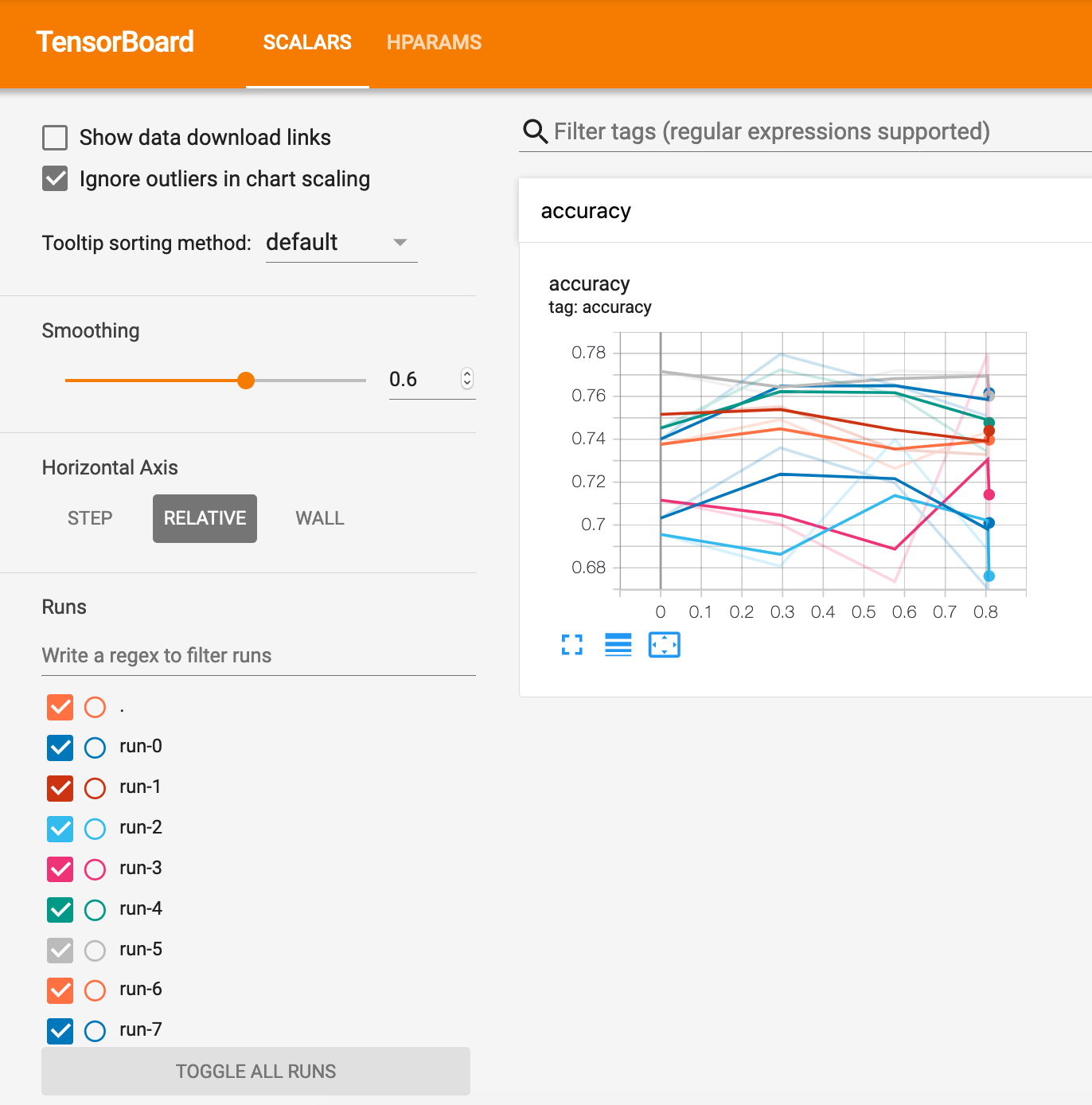

Challenge

There are a lot of parameters to adjust. For this challenge, try to reproduce the code exactly, either from the above or the link at the top and below. First, make sure you can get the Tensorboard running and then familiarize yourself with the output. Then, if you feel comfortable with that, try adjusting some of the parameters in the tuning function and see how they change the results.

Additional Resources

• Tensorboard: Tuning with hparams