Module 2: Train

Objective 01 - Explain the Intuition Behind Backpropagation and Gradient Descent

Overview

In the previous module, we learned more about the main components of neural networks, including neurons, weights, activation function, and the types of layers. We also created a simple perceptron binary classifier and an actual neural network using the Keras library. As we built those models, we focused more on the architecture, such as the number of layers and neurons in those layers. We also looked at parameters like the batch size and the learning rate and how they affect training time.

Now we're going to get more specific about how a neural network learns. First, we need to specify that we're talking about a feed-forward neural network, where information moves forward from the input. The weights are adjusted for each iteration; this process doesn't transfer data from one layer to the next inside the neural network.

In contrast, consider a multi-layer neural network where this transfer does occur. For example, if we added feedback from the last hidden layer to the first hidden layer, it would be considered a recurrent neural network (RNN), something we will cover in the next sprint.

Loss Function

So, what's going on when we train a neural network? First, remember to adjust the weights by comparing the model prediction with the expected result and adding or subtracting to those values to get closer to the correct answer. To do that, we minimize a loss function that compares the output to the target (correct answer). Using the process of gradient descent will minimize this function.

Gradient Descent

Given a function, in this case, the neural network loss function, we find the minimum of the function with the process of gradient descent. We start by choosing a random location on the function, finding the negative gradient's direction, and then repeat the process to find a minimum of the function. Sometimes, we find a local minimum, but the goal is to find the global minimum.

Follow Along

Let's work through an example with an actual function and find the minimum using gradient descent. The function we'll use is a simple parabola that has a single minimum.

y = (x-3)^2

Let's graph this function to see if we can see visually where the minimum is.

# Plot the function

import matplotlib.pyplot as plt
import numpy as np

x = np.arange(-10, 15, 0.01)
y = (x-3)**2

plt.plot(x, y)
plt.xlabel('x'); plt.ylabel('y')

plt.show()

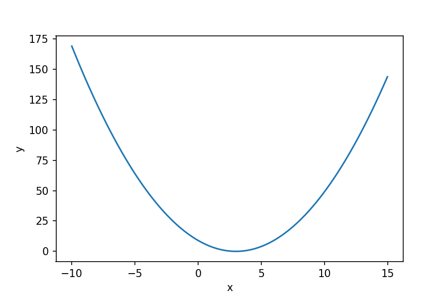
We can see it reaches a minimum (y=0) when x=3. Using calculus, we can find the minimum mathematically. We do this by looking at the slope of the function and finding when that slope is equal to zero. We find the slope by taking the derivative of the function. We'll take the derivative of y for x.

If we set the derivative equal to zero and solve for x, we'll have a solution for the minimum of the function:

0 = 2(x-3) which is true when x = 3.

Using Python, we'll implement a gradient descent function. First let's rewrite the equation as follows:

x{current} = (x{previous} - learning rate) * (dx/dy)

where dx/dy equals 2(x_previous-3).

The basic steps that we'll follow are:

• initialize at a value for x
• calculate a "new" current x with the learning rate and gradient
• update the next iteration with this "new" value of x
• iterate until the maximum number of iterations is reached

# Initialize at x=1
cur_x = 1 

# Learning rate (how much to adjust x each iteration)
rate = 0.05

# Maximum number of iterations
max_iters = 25

# Initialize interation counter
iters = 0

# Gradient of the function
grad = lambda x: 2*(x-3)

while iters < max_iters:
  # Set the previous x as the current
  prev_x = cur_x

  # Calculate the "new" current x with the gradient
  cur_x = prev_x - (rate * grad(prev_x))

  # Advance the iteration counter
  iters = iters+1
  print(f"Iteration {iters} - x value: {cur_x}")

# Print out the final result
print("The local minimum occurs at", cur_x)

Iteration 1 - x value: 1.2
Iteration 2 - x value: 1.38
Iteration 3 - x value: 1.5419999999999998
Iteration 4 - x value: 1.6877999999999997
Iteration 5 - x value: 1.8190199999999999
Iteration 6 - x value: 1.937118
Iteration 7 - x value: 2.0434061999999997
Iteration 8 - x value: 2.1390655799999996
Iteration 9 - x value: 2.2251590219999997
Iteration 10 - x value: 2.3026431198
Iteration 11 - x value: 2.37237880782
Iteration 12 - x value: 2.4351409270380002
Iteration 13 - x value: 2.4916268343342
Iteration 14 - x value: 2.54246415090078
Iteration 15 - x value: 2.5882177358107024
Iteration 16 - x value: 2.629395962229632
Iteration 17 - x value: 2.6664563660066687
Iteration 18 - x value: 2.6998107294060016
Iteration 19 - x value: 2.7298296564654017
Iteration 20 - x value: 2.7568466908188616
Iteration 21 - x value: 2.7811620217369755
Iteration 22 - x value: 2.8030458195632777
Iteration 23 - x value: 2.82274123760695
Iteration 24 - x value: 2.840467113846255
Iteration 25 - x value: 2.8564204024616293
The local minimum occurs at 2.8564204024616293

After 25 iterations, the value is starting to converge on the minimum of x=3. To speed up the convergence, we can adjust the learning rate or the size of the step we adjust x by. We'll leave that up to you to complete as a challenge.

Challenge

Following the example above, try experimenting with the gradient descent algorithm. Specifically, you can change the learning rate and adjust the maximum number of iterations. How close can you get to the minimum value of the function?

Additional Resources

• Khan Academy: Gradient and Directional Derivatives
• Implement a Gradient Descent in Python

Objective 02 - Discuss the Importance of Batch Size

Overview

You may have noticed one of the parameters when we fit our models were "batch size." Now we're going to pay attention to what this parameter means and get a start on what values it should have.

What is a Batch?

When training a neural net, a given number of samples or a batch is used to make predictions, calculate the error, and update the weights. During one epoch, the weights are updated for each batch.

Let's look at an example where we have 2000 training samples. If we set the batch size to be 100, during each epoch, a batch of 100 samples is selected randomly, the error calculated, and the weights updated. Then, the next batch is selected, weights updated, and all the samples are used. Then, the next epoch starts with the same batch-selection process.

Choosing Batch Size

The batch size is vital for a few reasons. First, smaller batch sizes require less memory because you don't need to hold the whole dataset in memory. Second, neural networks also can train faster using smaller batches. But smaller batch sizes can be less accurate because the smaller samples make it more difficult to calculate the error gradient.

In the end, it's a balance between choosing a large enough batch size to represent your data but not too large that the training time is too long and the memory use too high.

Let's look at an example with a real dataset and see what happens when we change the batch size.

Follow Along

Using the Pima Indians health dataset we used from the previous module, we'll try out a few different batch sizes and look at the accuracy. Since we're using a relatively small dataset for this example, we can use a larger batch size that won't give us any problems storing in memory.

# Load the Pima Indians diabetes dataset
import numpy as np

# Set the URL for the data location
url = 'https://raw.githubusercontent.com/jbrownlee/Datasets/master/pima-indians-diabetes.data.csv'

# Load the dataset
dataset = np.loadtxt(url, delimiter=',')

# Look at the size of the dataset
print(f"There are {len(dataset)} samples in this dataset.")

# Split into input (X) and output (y) variables
# (8 input columns, 1 target column)
X = dataset[:,0:8]
y = dataset[:,8]

# Import keras
import tensorflow as tf
from keras.models import Sequential
from keras.layers import Dense

# Define the layers
model = Sequential()
model.add(Dense(12, input_dim=8, activation='relu'))
model.add(Dense(8, activation='relu'))
model.add(Dense(1, activation='sigmoid'))

# Compile the model
model.compile(loss='binary_crossentropy', optimizer='adam', metrics=['accuracy'])

There are 768 samples in this dataset.

Now we'll fit the model with different batch sizes. It will be faster to do these one at a time rather than in a loop so that we can more easily adjust the batch size without running the whole loop each time.

We'll start with a batch size of 1 which means each sample will determine how to update the weights in the layer.

# Define batch sizes
size = 1

# Fit the model with different batch sizes
model.fit(X, y, epochs=100, batch_size=size, verbose=0)

# Evaluate the model
print(f'Model accuracy for batch size = {size}: ', model.evaluate(X, y)[1]*100)

24/24 [==============================] - 0s 968us/step - loss: 0.5355 - accuracy: 0.7122
Model accuracy for batch size = 1:  71.22395634651184

This is a pretty high accuracy but because we are using such a small sample size, it's possible that we could be overfitting the model. Next, we'll increase the batch size to an intermediate value; let's try 100.

# Release global memory state
tf.keras.backend.clear_session()

# Define the layers
model = Sequential()
model.add(Dense(12, input_dim=8, activation='relu'))
model.add(Dense(8, activation='relu'))
model.add(Dense(1, activation='sigmoid'))

# Compile the model
model.compile(loss='binary_crossentropy', optimizer='adam', metrics=['accuracy'])

# Define batch sizes
size = 100

# Fit the model with different batch sizes
model.fit(X, y, epochs=100, batch_size=size, verbose=0)

# Evaluate the model
print(f'Model accuracy for batch size = {size}: ', model.evaluate(X, y)[1]*100)

24/24 [==============================] - 0s 913us/step - loss: 0.5435 - accuracy: 0.7344
Model accuracy for batch size = 100:  73.4375

The accuracy has decreased for a larger batch size, which isn't necessarily bad. Finally, we'll use the largest batch size available: the length of the training data set.

# Release global memory state
tf.keras.backend.clear_session()

# Define the layers
model = Sequential()
model.add(Dense(12, input_dim=8, activation='relu'))
model.add(Dense(8, activation='relu'))
model.add(Dense(1, activation='sigmoid'))

# Compile the model
model.compile(loss='binary_crossentropy', optimizer='adam', metrics=['accuracy'])


# Define batch sizes
size = len(X)

# Fit the model with different batch sizes
model.fit(X, y, epochs=100, batch_size=size, verbose=0)

# Evaluate the model
print(f'Model accuracy for batch size = {size}: ', model.evaluate(X, y)[1]*100)

24/24 [==============================] - 0s 1ms/step - loss: 0.9863 - accuracy: 0.6133
Model accuracy for batch size = 768:  61.328125

As we expected, the accuracy has decreased because we're using the whole data set as a batch. In addition, the error in the model is only updated once per epoch, so there are fewer opportunities for the model to adjust the error and learn a better fitting model.

Because extensive datasets are often used to train deep learning neural networks, the batch size is rarely set to the training set size. Usually, smaller batch sizes improve the model's generalization (fitting or generalizing to new data). A recommended starting point for batch sizes is between n=2 and n=32.

Challenge

You should try to reproduce the code above (just for a single batch size). Try changing the batch size yourself or looping over a list of batch sizes. You will need to clear the model between batch sizes; you can do this with keras.backend.clear_session().

Additional Resources

• Revisiting Small Batch Training for Deep Neural Networks (arXiv paper)
• How to Control the Stability of Training Neural Networks With the Batch Size

Objective 03 - Discuss the Importance of Learning Rate

Overview

In the first objective in this module, we implemented a very basic gradient descent using Python. Remember the part we set as the learning rate? It was the amount by which x was adjusted in each iteration.

In a neural network, the learning process happens by calculating the error in the prediction and then adjusting the weight to reduce this error. Thus, the loss function calculates the error, and we want to find the minimum in the loss function.

The learning rate specifies how much we jump around on this loss function. Big jumps (large learning rate) might not allow convergence toward the minimum error. Small jumps (small learning rate) may result in a long convergence time. Selecting the appropriate learning rate for a given neural network is somewhat of a trial-and-error process.

Follow Along

Similar to how we tested different batch sizes, we'll look at different learning rates to see how they affect the accuracy. Because we have a smaller dataset, we don't need to pay as much attention to how long it takes to train the model, but it's an important consideration with a larger dataset.

# Load the Pima Indians diabetes dataset
import numpy as np

# Set the URL for the data location
url = 'https://raw.githubusercontent.com/jbrownlee/Datasets/master/pima-indians-diabetes.data.csv'

# Load the dataset
dataset = np.loadtxt(url, delimiter=',')

# Look at the size of the dataset
print(f"There are {len(dataset)} samples in this dataset.")

# Split into input (X) and output (y) variables
# (8 input columns, 1 target column)
X = dataset[:,0:8]
y = dataset[:,8]

# Split into training and test sets
from sklearn.model_selection import train_test_split

X_train, X_test, y_train, y_test = train_test_split(
    X, y, test_size=0.25, random_state=42)

There are 768 samples in this dataset.

# Import keras
import tensorflow as tf
from keras.models import Sequential
from keras.layers import Dense
from keras.optimizers import SGD

# Define the layers
model = Sequential()
model.add(Dense(12, input_dim=8, activation='relu'))
model.add(Dense(8, activation='relu'))
model.add(Dense(1, activation='sigmoid'))

# Compile the model
opt = SGD(lr=0.0001)
model.compile(loss='binary_crossentropy', optimizer=opt, metrics=['accuracy'])

# Fit the model with validation data
lr_low = model.fit(X_train, y_train, epochs=50, batch_size=10, verbose=0,
                       validation_data=(X_test, y_test))

# Evaluate the model
print('Model accuracy for learning rate = 0.0001:', model.evaluate(X, y)[1]*100)

24/24 [==============================] - 0s 1ms/step - loss: 0.7017 - accuracy: 0.6406
Model accuracy for learning rate = 0.0001: 64.0625

# Release global memory state
tf.keras.backend.clear_session()

# Define the layers
model = Sequential()
model.add(Dense(12, input_dim=8, activation='relu'))
model.add(Dense(8, activation='relu'))
model.add(Dense(1, activation='sigmoid'))

# Compile the model
opt = SGD(lr=0.75)
model.compile(loss='binary_crossentropy', optimizer=opt, metrics=['accuracy'])

# Fit the model with different batch sizes
lr_high = model.fit(X_train, y_train, epochs=50, batch_size=10, verbose=0,
                       validation_data=(X_test, y_test))

# Evaluate the model
print('Model accuracy for learning rate = 0.75:', model.evaluate(X, y)[1]*100)

24/24 [==============================] - 0s 2ms/step - loss: 0.6580 - accuracy: 0.6510
Model accuracy for learning rate = 0.75: 65.10416865348816

We trained two models, one with a low learning rate and one with a high learning rate. We saved each model and can use the history method to look at the loss and accuracy values for each epoch. Using this data, we can plot the loss (top plot).

# Import plotting libraries and pandas
import pandas as pd

# Create an empty list to append each DataFrame
learn_rates = []

# Loop through the history of each model and create a DataFrame
for model, result in zip([lr_low, lr_high], ["0.0001_", "0.75_"]):
  df = pd.DataFrame.from_dict(model.history)
  df['epoch'] = df.index.values
  df['Learning Rate'] = result
  learn_rates.append(df)

# Combine all the DataFrames
df = pd.concat(learn_rates)
df['Learning Rate'] = df['Learning Rate'].astype('str')
df.head()

   loss  accuracy   val_loss  val_accuracy  epoch Learning Rate
0  2.212333  0.571181  1.386622  0.473958  0  0.0001_
1  1.232326  0.505208  1.630090  0.463542  1  0.0001_
2  1.156209  0.546875  1.117308  0.541667  2  0.0001_
3  1.033138  0.553819  1.134055  0.567708  3  0.0001_
4  0.994407  0.574653  0.997309  0.562500  4  0.0001_

# Create the plot
import matplotlib.pyplot as plt
import seaborn as sns

fig, (ax1, ax2) = plt.subplots(1, 2, figsize=(12,6))
sns.lineplot(x='epoch', y='val_loss', hue='Learning Rate', data=df, ax=ax1)
sns.lineplot(x='epoch', y='val_accuracy', hue='Learning Rate', data=df, ax=ax2);

fig.show()

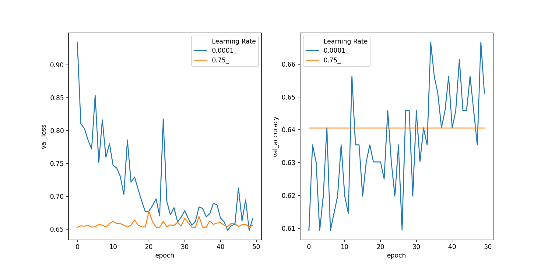
Let's take a quick look at these plots. As we expected, it takes longer for the slower learning rate to decrease the loss function compared to the higher learning rate. The validation accuracy also bounces around a lot compared to the lower learning rate, but it eventually finds a higher validation accuracy. There is much less variation for the higher learning rate: it finds weights quickly and doesn't change much. But, the accuracy is lower than we found with the lower learning rate.

Selecting the best learning rate can be a process of trial and error. There are a few tools in Keras that we haven't covered that we can use to select the best learning rate and even adjust the learning rate during the model fitting process.

Challenge

Using either the same dataset as above or a different dataset, try using different learning rates. Store the history of your model and reproduce the plots, but with varying rates of learning. Were you able to find a happy medium or a learning rate that was better with this dataset?

Additional Resources

• Keras: learning rate scheduler
• Understand the Dynamics of Learning Rate on Deep Learning Neural Networks