Module 4: Classification Metrics
Module Overview
This last module will cover some important concepts in Data Science including classification model evaluation metrics. We'll introduce a confusion matrix along with how to interpret precision and recall. Additionally, we'll learn about the receiver operating characteristic (ROC) curve and how we can use it to interpret a classifier model.
Learning Objectives
- Get & interpret Confusion Matrix
- Use Precision and Recall
- Understand relationships between classification thresholds, metrics and predicted probabilities
Objective 01 - get and interpret the confusion matrix for classification models
Overview
When we evaluate a model we are often looking at a score, such as the accuracy for a classification model. When we are using a classifier however, it's helpful to evaluate a model visually. The plot of the confusion matrix is easy to interpret and see where the model may have gone wrong and why. This helps to identify patterns in misclassification.
The confusion matrix is often plotted as a heatmap where the columns represent the predicted class and the rows represent the true classes. The diagonal of the matrix should be equal to the total number of correct predictions for each class (or ones if the matrix is normalized by the number of observations. A confusion matrix works for any number of classes, but the plot would start to become less useful with a very large number of classes.
Follow Along
We used the digits data set for computing and displaying the confusion matrix.
In the lecture recordings, plot_confusion_matrix function was used. This is deprecated in
sklearn 1.0
and will be removed in 1.2. Here we will use the ConfusionMatrixDisplay.from_estimator
class method to
build our confusion matrix. Alternatively, ConfusionMatrixDisplay.from_predictions can also
be used.
# Import necessary modules
import numpy as np
import pandas as pd

from sklearn import datasets
from sklearn.model_selection import train_test_split
from sklearn.tree import DecisionTreeClassifier
from sklearn.metrics import ConfusionMatrixDisplay
# Load the digits data
# The default with 10 classes (digits 0-9)
digits = datasets.load_digits(n_class=10)
# Create the feature matrix
X = digits.data
# Create the target array
y = digits.target
# Split the data into a training set and a test set
X_train, X_test, y_train, y_test = train_test_split(X, y, random_state=0)
# Instantiate and train a decision tree classifier
dt_classifier = DecisionTreeClassifier().fit(X_train, y_train)# plot the confusion matrix
import matplotlib.pyplot as plt
ConfusionMatrixDisplay.from_estimator(dt_classifier, X_test, y_test)
plt.show()<Figure size 576x576 with 0 Axes>
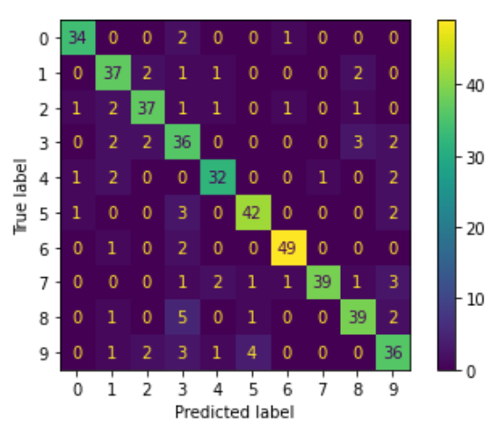
In this confusion matrix we can see that the model performs well. There are a few numbers though that the
model has more trouble with. Can you identify those? For example, the model was incorrect when trying to
distinguish between a 2 and a 3. The model was incorrect when trying to
distinguish between a 2 and a 3
and also between a 4 and a 7.
Challenge
For this challenge, try using a different data set for which to plot the confusion matrix. The Iris data set is pretty common, but you could also use one of the data sets that we have worked with previously such as the penguin data set. You can also compare what the confusion matrix looks like for a different classifier. In the above example, we use a decision tree but you could try a logistic regression classifier.
Additional Resources
Objective 02 - use the classification metrics of precision and recall
Overview
For some data sets and models simply calculating the accuracy is often not enough. If for example, your data set has imbalanced classes (measuring disease occurrence or other uncommon events) then you might have an excellent accuracy score that isn't actually a useful metric. This objective will focus on the concepts of precision and recall.
Precision is the portion of positive classifications that were actually correct. It can be calculated by the following equation:
where is the number
of true positives and
is the number of false positives. A false positive is
where an observation is predicted to belong to a class but isn't actually of that class.
The other metric that is useful in evaluation of classification models is the recall or portion of actual positives that were identified correctly. This value is calculated by:
where is the number
of
true
positives and
is the number of
false
negatives. A false negative is
where in observation is not predicted to belong to a certain class but actually is of that class.
There is a balance between precision and recall: often by improving one value, the other value decreases. In other words, if we reduce the number of false positives (by improving our model), the precision will increase. But fewer false positives results in more false negatives, which decreases the recall value.
A value that takes into consider both precision and recall is called the F1 score, or sometimes just the F-score. It is calculated by:
Follow Along
Let's use the information above to interpret the confusion matrix for the digits data set. To make the interpretation more simple, we'll use only some of the digits. We'll also limit the depth of the tree so that the model isn't as good as it could be. This way, we'll get some false positives and false negatives.
# Import necessary modules
import numpy as np
import pandas as pd

from sklearn import datasets, metrics
from sklearn.model_selection import train_test_split
from sklearn.tree import DecisionTreeClassifier
from sklearn.metrics import ConfusionMatrixDisplay
# Load the digits data
# Use the first four digits (0-3)
digits = datasets.load_digits(n_class=4)
# Create the feature, target
X = digits.data
y = digits.target
# Split the data into a training set and a test set
X_train, X_test, y_train, y_test = train_test_split(X, y, random_state=0)
# Instantiate and train a decision tree classifier
dt_classifier = DecisionTreeClassifier(max_depth=3).fit(X_train, y_train)# Plot the decision matrix
import matplotlib.pyplot as plt
fig, ax = plt.subplots(1,1,figsize=(8,8))
#plot the confusion matrix
import matplotlib.pyplot as plt
ConfusionMatrixDisplay.from_estimator(dt_classifier, X_test, y_test)
plt.show()<Figure size 576x576 with 0 Axes>
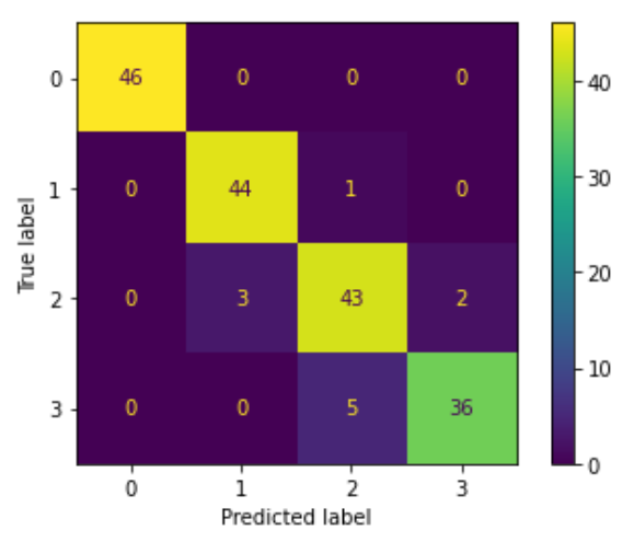
We can see the model had a little difficulty with 2 and 1. 1 was
predicted three times but the true label
was a 2. And we see something similar with 2 and 3 where
2 was predicted five times but the true label
was 3.
Instead of calculating the precision and recall for all of these features, we can use the scikit-learn
classification_report function to calculate and display everything for us. The f1-score is
also returned
in this report.
y_pred = dt_classifier.predict(X_test)
print (metrics.classification_report(y_test, y_pred))
              precision    recall  f1-score   support

           0       1.00      1.00      1.00        46
           1       0.94      0.98      0.96        45
           2       0.88      0.90      0.89        48
           3       0.95      0.88      0.91        41

    accuracy                           0.94       180
   macro avg       0.94      0.94      0.94       180
weighted avg       0.94      0.94      0.94       180
Challenge
With the code above try fitting a classification model to a different data set and plot both the confusion matrix and return the classification report.
Additional Resources
Objective 03 - understand the relationships between precision, recall, thresholds, and predicted probabilities
Overview
When fitting a classification model, one thing we haven't discussed very much is the classification threshold, or the value at which we decide if an observation belongs in one class or the other. This concept is also tied to the probability of each observation belonging to that class. By default, scikit-learn predicts an observation is part of the class if the probability is greater than 0.5 (this is the threshold).
There might be some situations where using a different probability threshold is important. For example, in a medical study using very expensive medication with very negative side effects, it might be necessary to set the probability threshold much higher than 0.5 to classify a patient as needing the medication. In this case, the medication should only be used if the patient has a high probability of belonging to a class that needs the treatment.
In the following example we'll use scikit-learn to create a classification data set and look at the predicted probabilities.
Follow Along
# Load modules
from sklearn.datasets import make_classification
from sklearn.linear_model import LogisticRegression
from sklearn.model_selection import train_test_split

# Create the data (feature, target)
X, y = make_classification(n_samples=10000, n_features=5,
                          n_classes=2, n_informative=3,
                          random_state=42)

# Split the data into a training set and a test set
X_train, X_test, y_train, y_test = train_test_split(X, y, random_state=42)

# Create and fit the model
logreg_classifier = LogisticRegression().fit(X_train, y_train)
Now that we have created the data set and fit the model, let's look at the target probabilities. We can
use the method predict_proba() with our test data. We'll look at a single prediction and
interpret the probability.
# The value of the 10th observation
print('The 10th observation: ', X_test[10:11])
# Print out the probability for the 10th observation
print('Predicted probability for the 10th observation: ',
      logreg_classifier.predict_proba(X_test)[10:11])
# Print the two classes
print('The two classes: ')
logreg_classifier.classes_
The 10th observation:  [[-0.73552378  1.05914888 -0.60278934 -0.32282208  0.55717004]]
Predicted probability for the 10th observation:  [[0.73592057 0.26407943]]
The two classes:

array([0, 1])
This observation has a 74% chance of belonging to the first class and a 26% chance of belonging in the
second class. Is it actually in the first class (0)? Let's take a look.
# Check the class of the 10th observation
logreg_classifier.predict(X_test[10:11])
array([0])
The 10th observation was predicted to be in the first class (0) and it was. In the next
objective, we're
going to look at how we extend this single observation into something called a receiver operating
characteristic or ROC curve.
Challenge
With the example data set above, look at a few other observations. Take a look at their class and the predicted probability of being in that class. Are they all correct? Spoiler: Yes.
Additional Resources
Guided Project
Open JDS_SHR_224_guided_project_notes.ipynb in the GitHub repository below to follow along with the guided project:
Guided Project Video
Module Assignment
Complete the Module 4 assignment to practice classification metrics techniques you've learned.
In this module assignment, you'll continue working with the Tanzania Waterpumps Kaggle competition: